How to sum up working hours (a different schedule)

[KarolinaKaralaite]

Hello,

I'm kinda new to excel and there is soooo many thingies in here... I've been spending days to figure out the problems in my formulas on my own but I got really stuck now...

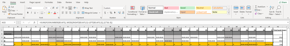
So at first I was really happy that I was able to find formula and make it work for two rows of my employees (A and B). The formula I used was:

=SUM(IF(ISBLANK(B3:AF3),"",(MOD((RIGHT(B3:AF3,5)-LEFT(B3:AF3,5)),1)*24)))

But my employee "C" (5th row) has holidays for 10 days and I write them down as a letter "H" (stands for holiday). So I tried numerous formulas instead of ISBLANK like IFERROR or ISNUMBER but i still get #VALUE! or a 0:00. I even added additional letters like "P" (that stands for off day.). I thought if I remove all blank cells and make it only letters (cells with text in other words) I could make a certain formula to count hours. So to say I want a formula that it would ignore text but if its a number - that it would count hours.

My latest formula for this at AG5 for employee C was:
=SUM(IF(ISNUMBER(B5:AF5), MOD((RIGHT(B5:AF5,5)-LEFT(B5:AF5,5)),1)*24, 0))

But of course it gives me 0:00 value.

This timetable is for nurses that work in hospital 24h shifts, day shifts (11 hours), night shifts (13 hours) and additional hours if needed.

Can somebody help me to figure this formula out?

 

[KarolinaKaralaite]

Forgot to mention that this is whole October month I try to calculate hours for. Also I will try to upload mini-sheet.

Spalio darbo grafikas Bandymas slaugytojos.xlsx
	A	B	C	D	E	F	G	H	I	J	K	L	M	N	O	P	Q	R	S	T	U	V	W	X	Y	Z	AA	AB	AC	AD	AE	AF	AG
1		1	2	3	4	5	6	7	8	9	10	11	12	13	14	15	16	17	18	19	20	21	22	23	24	25	26	27	28	29	30	31	Total work hours
2	Darbuotojai
3	A	08:00-24:00	00:00-08:00			08:00-24:00	00:00-08:00			08:00-24:00	00:00-08:00			08:00-24:00	00:00-08:00			08:00-24:00	00:00-08:00			08:00-24:00	00:00-08:00			08:00-24:00	00:00-08:00			08:00-14:48			174.8
4	B		08:00-24:00	00:00-08:00			08:00-24:00	00:00-08:00			08:00-24:00	00:00-08:00			08:00-24:00	00:00-08:00			08:00-24:00	00:00-08:00		08:00-19:00			19:00-24:00	00:00-08:00			08:00-14:48	08:00-24:00	00:00-08:00		174.8
5	C	P	P	08:00-24:00	00:00-08:00	P	P	08:00-24:00	00:00-08:00	P	P	19:00-24:00	00:00-08:00	P	H	H	H	H	H	P	P	H	H	H	H	H	P	P	08:00-24:00	00:00-08:00	P	08:00-17:48	0:00
Sheet1

Cell Formulas
Range	Formula
AG3:AG4	AG3	=SUM(IF(ISBLANK(B3:AF3),"",(MOD((RIGHT(B3:AF3,5)-LEFT(B3:AF3,5)),1)*24)))
AG5	AG5	=SUM(IF(ISNUMBER(B5:AF5), MOD((RIGHT(B5:AF5,5)-LEFT(B5:AF5,5)),1)*24, 0))

 

[RobP]

Hi,

going back to your original formula, you could use the OR() statement as your first check, as such perhaps ?

=SUM(IF(OR(ISBLANK(B3:AF3),B3:AF3="H",B3:AF3="P"),"",(MOD((RIGHT(B3:AF3,5)-LEFT(B3:AF3,5)),1)*24)))

 

[KarolinaKaralaite]

Hi,

going back to your original formula, you could use the OR() statement as your first check, as such perhaps ?

=SUM(IF(OR(ISBLANK(B3:AF3),B3:AF3="H",B3:AF3="P"),"",(MOD((RIGHT(B3:AF3,5)-LEFT(B3:AF3,5)),1)*24)))

I tried your formula but it shows again #VALUE!
Checked several times if I wrote it correctly

 

[KarolinaKaralaite]

I tried your formula but it shows again #VALUE!
Checked several times if I wrote it correctly

I did change it ranges to b5:af5 thow cuz its fifth row but all the rest the same as you wrote

 

[RobP]

sorry I hadn't tested it fully on your sheet .. will try again !

 

[RobP]

maybe this one :

=SUM(IFERROR(MOD((RIGHT(B3:AF3,5)-LEFT(B3:AF3,5)),1)*24,0))

 

[KarolinaKaralaite]

THANK YOU OMG IT WORKED. I WAS TRYING TO FIGURE THIS OUT FOR 3 DAYS haha... I'm almost crying.

Thank you and big loves from me!

 

[RobP]

your welcome, thanks for the feedback.

you had done the hard work in working out how to get your hours. then just break your formula down to see what its actually doing at each stage as such :

Book1
	B	C	D	E	F	G	H	I	J	K	L	M	N	O	P	Q	R	S	T	U	V	W	X	Y	Z	AA	AB	AC	AD	AE	AF
9	16	8	#VALUE!	#VALUE!	16	8	#VALUE!	######	16	8	#VALUE!	#VALUE!	16	8	#VALUE!	#VALUE!	16	8	#VALUE!	#VALUE!	16	8	#VALUE!	#VALUE!	16	8	#VALUE!	#VALUE!	6.8	#VALUE!	#VALUE!
10	16	8	0	0	16	8	0	0	16	8	0	0	16	8	0	0	16	8	0	0	16	8	0	0	16	8	0	0	6.8	0	0
11	174.8
12
Sheet1

Cell Formulas
Range	Formula
B9:AF9	B9	=MOD((RIGHT(B3:AF3,5)-LEFT(B3:AF3,5)),1)*24
B10:AF10	B10	=IFERROR(MOD((RIGHT(B3:AF3,5)-LEFT(B3:AF3,5)),1)*24,0)
B11	B11	=SUM(IFERROR(MOD((RIGHT(B3:AF3,5)-LEFT(B3:AF3,5)),1)*24,0))
Dynamic array formulas.

Rob

 

[KarolinaKaralaite]

your welcome, thanks for the feedback.

you had done the hard work in working out how to get your hours. then just break your formula down to see what its actually doing at each stage as such :

Book1
	B	C	D	E	F	G	H	I	J	K	L	M	N	O	P	Q	R	S	T	U	V	W	X	Y	Z	AA	AB	AC	AD	AE	AF
9	16	8	#VALUE!	#VALUE!	16	8	#VALUE!	######	16	8	#VALUE!	#VALUE!	16	8	#VALUE!	#VALUE!	16	8	#VALUE!	#VALUE!	16	8	#VALUE!	#VALUE!	16	8	#VALUE!	#VALUE!	6.8	#VALUE!	#VALUE!
10	16	8	0	0	16	8	0	0	16	8	0	0	16	8	0	0	16	8	0	0	16	8	0	0	16	8	0	0	6.8	0	0
11	174.8
12
Sheet1

Cell Formulas
Range	Formula
B9:AF9	B9	=MOD((RIGHT(B3:AF3,5)-LEFT(B3:AF3,5)),1)*24
B10:AF10	B10	=IFERROR(MOD((RIGHT(B3:AF3,5)-LEFT(B3:AF3,5)),1)*24,0)
B11	B11	=SUM(IFERROR(MOD((RIGHT(B3:AF3,5)-LEFT(B3:AF3,5)),1)*24,0))
Dynamic array formulas.

Rob

thank you for recomendation I will use this formula"dividing" tip in the future problems!