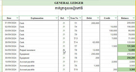
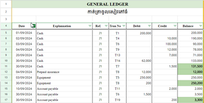
How to set bold on text on cell of last row by each category?

[Son Raphon]

Dear all, I have a table that separated item by category. I want to set bold text on last cell of row by using conditional formatting.
Example: I have Col Item name and Col Amount.
Item Name, Amount
A 100
A 200,
A 300
B 50
B 100

I want to set bold on col amount with 300 for category A.
And set bold on col amount with 100 for category B.

Anyone, could you guide and help me?

 

[Cubist]

This is for category A. Here I assumed the last row is 5, but adjust to the actual range.

=AND($A1="A", $B1=MAX(IF($A$1:$A$5="A", $B$1:$B$5)))

...and this is for category B.

=AND($A1="B", $B1=MAX(IF($A$1:$A$5="B", $B$1:$B$5)))

 

[Son Raphon]

This is for category A. Here I assumed the last row is 5, but adjust to the actual range.

=AND($A1="A", $B1=MAX(IF($A$1:$A$5="A", $B$1:$B$5)))

...and this is for category B.

=AND($A1="B", $B1=MAX(IF($A$1:$A$5="B", $B$1:$B$5)))

Thanks you so much for your helping.
I try to apply my task. I doesn't work correctly.
I will send by image of my task. I want to get result like this.

FYI. I'm a student of university.

 

[Son Raphon]

I forgot to show column number.
I send image again.

 

[Cubist]

Edit:
I realized you wanted the last row of each category instead of the max amount. Try this.

Book1
	A	B
1	A	1
2	A	2
3	A	1
4	B	1
5	B	0
Sheet4

Cells with Conditional Formatting
Cell	Condition		Cell Format	Stop If True
B1:B5	Expression	=AND($A1="A", COUNTIF($A$1:$A$5,"A")=COUNTIF($A$1:$A1,"A"))	text	NO
B1:B5	Expression	=AND($A1="B", COUNTIF($A$1:$A$5,"B")=COUNTIF($A$1:$A1,"B"))	text	YES

 

[Son Raphon]

Edit:
I realized you wanted the last row of each category instead of the max amount. Try this.

Book1
	A	B
1	A	1
2	A	2
3	A	1
4	B	1
5	B	0
Sheet4

Cells with Conditional Formatting
Cell	Condition		Cell Format	Stop If True
B1:B5	Expression	=AND($A1="A", COUNTIF($A$1:$A$5,"A")=COUNTIF($A$1:$A1,"A"))	text	NO
B1:B5	Expression	=AND($A1="B", COUNTIF($A$1:$A$5,"B")=COUNTIF($A$1:$A1,"B"))	text	YES

It showed the result as in image.
Could you help to check?

 

[Cubist]

You have one too many $ sign. Remove the last $.

 

[Son Raphon]

I forgot to show column name.

 

[Son Raphon]

Keep like this?
=AND($V5="Cash", COUNTIF($V5:$V50,"Cash")=COUNTIF($V5:$V50,"Cash"))

 

[Cubist]

Just the very last one.

=AND($V5="Cash", COUNTIF($V$5:$V$50,"Cash")=COUNTIF($V$5:$V50,"Cash"))