How to look up data from on sheet to another when both sheets have multiple cells with the same ID number.

[lil_Sassy]

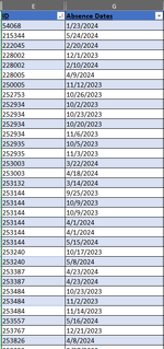
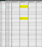
I can't add a mini sheet because my company has protective view enabled and I can't deselect it. I added pictures in hopes this will help.

I have to track information for my company for team members for dates missed pertaining to a leaves of absence. I have input the information form the absences form into a tracking sheet. (Sheet A Image) So, there are team members with multiple dates on this sheet. and same IDs multiple times I then receive a list that has the approved/denied absences dates and amount of time. (Image Sheet B) This sheet also has team members listed multiple times with different dates. I want to have Sheet A look at Sheet B and tell me who was approved or denied and what those date/s are and the amount of time.

I need to look at columns E, G in sheet A. The ID and date and then look at sheet B and see if that ID is in column B and same date in Column E, if so look at Columns G, H, I and get those amounts. Results Image is what I am looking for in Columns D & E.

Same IDs in both sheets multiple times. I don't know how to set up a formula to decipher all of this, or if it can be done or if there is some other way to obtain this. I just don't want to check 1300 IDs in a sheet manually.
If I need to send a mock file another way, I can.

 

[hagia_sofia]

Would this work for if you adjust ranges based on your data:

=LET(
array,TRANSPOSE(VSTACK('Sheet B'!$G$1:$I$1,FILTER('Sheet B'!$G$2:$I$100,('Sheet B'!$D$2:$D$100=E2)*('Sheet B'!$E$2:$E$100=G2),0))),
IFERROR(SUBSTITUTE(FILTER(array,CHOOSECOLS(array,2)<>0),"Hours",""),"NO ABSENCE"))

 

[lil_Sassy]

Would this work for if you adjust ranges based on your data:

=LET(
array,TRANSPOSE(VSTACK('Sheet B'!$G$1:$I$1,FILTER('Sheet B'!$G$2:$I$100,('Sheet B'!$D$2:$D$100=E2)*('Sheet B'!$E$2:$E$100=G2),0))),
IFERROR(SUBSTITUTE(FILTER(array,CHOOSECOLS(array,2)<>0),"Hours",""),"NO ABSENCE"))

Do I choose something for the "array" part in the formula? I am not this advanced with formulas, but I am trying to decipher it out.

 

[hagia_sofia]

Do I choose something for the "array" part in the formula? I am not this advanced with formulas, but I am trying to decipher it out.

No, just select those ranges, where there are columns and rows references.

 

[lil_Sassy]

No, just select those ranges, where there are columns and rows references.

Thank you for your help. I just don't understand how to make the formula work.

 

[hagia_sofia]

I presume that you have a list of a list of IDs and Absence dates on "Sheet A" and "Sheet 2" that corresponds to the one above. If it is so, then you need to select your ranges, where:

'Sheet B'!$G$1:$I$1 = headers, i.e. "Pending Hours", "Approved Hours", and "Denied Hours",
'Sheet B'!$G$2:$I$100 = range of values. i.e. hours (be it Pending, Approved, or Denied, i.e. all three columns),
'Sheet B'!$D$2:$D$100 = list of IDs on Sheet B,
E2 = an ID you are looking for on Sheet A,
'Sheet B'!$E$2:$E$100 = list of dates on Sheet B,
G2 = a date you are looking for on Sheet A

the rest is just calculation.