how to get a number based on a color

[streamer1234]

Hey,

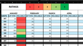
so I'm trying to figure out how to get a number based off a percentage to match with a color, if that makes sense lol.

ex: 0% to 20% = 1
21%-40% = 2
41% to 60% = 3
61% to 80% = 4
90% to 100% = 5

i have the conditional formatting a color scale already based of the percentage but cant figure out how to get a number to associate to it.

I've attached a photo to give an idea, please help lol

thanks - A

 

[Sergius]

Is this what you wanted? If so, replace the color with your own.

Book1
	B	C
4	0,00%
5	0,00%
6	40,00%
7	0,00%
8	80,00%
9	50,00%
10	95,00%
Sheet1

Cells with Conditional Formatting
Cell	Condition		Cell Format	Stop If True
C4:C10	Expression	=$B4<=20%	text	NO
C4:C10	Expression	=$B4<=40%	text	NO
C4:C10	Expression	=$B4<=60%	text	NO
C4:C10	Expression	=$B4<=80%	text	NO
C4:C10	Expression	=$B4<=100%	text	NO

 

[streamer1234]

yea something like that but the " text" section is numbers 1-5, and how and where would i write it

 

[streamer1234]

i was wanting the numbers to be in column E, which would be equivalent to the colors in D

 

[Sergius]

These are conditional formatting rules (see the photo).

 

[streamer1234]

These are conditional formatting rules (see the photo).
View attachment 120537

yes i already have that section done, what im trying to do is if its red in column C4, it would place #1 in C4, and if its yellow in c11 then it would but a 3 in the same spot. so even if the numbers go up or down itll match color to the formula plus have the correct # to the color, like a rating

 

[Sergius]

Is this what you wanted?

mrexcel.xlsx
	B	C	D	E	F	G	H
1			1	2	3	4	5
2
3
4	0,00%	1
5	0,00%	1
6	40,00%	2
7	0,00%	1
8	80,00%	4
9	50,00%	3
10	95,00%	5
Sheet1

Cell Formulas
Range	Formula
C4:C10	C4	=IFS($B4<=20%,$D$1,$B4<=40%,$E$1,$B4<=60%,$F$1,$B4<=80%,$G$1,$B4<=100%,$H$1)

Cells with Conditional Formatting
Cell	Condition		Cell Format	Stop If True
C4:C10	Expression	=$B4<=20%	text	NO
C4:C10	Expression	=$B4<=40%	text	NO
C4:C10	Expression	=$B4<=60%	text	NO
C4:C10	Expression	=$B4<=80%	text	NO
C4:C10	Expression	=$B4<=100%	text	NO

 

[streamer1234]

Is this what you wanted?

mrexcel.xlsx
	B	C	D	E	F	G	H
1			1	2	3	4	5
2
3
4	0,00%	1
5	0,00%	1
6	40,00%	2
7	0,00%	1
8	80,00%	4
9	50,00%	3
10	95,00%	5
Sheet1

Cell Formulas
Range	Formula
C4:C10	C4	=IFS($B4<=20%,$D$1,$B4<=40%,$E$1,$B4<=60%,$F$1,$B4<=80%,$G$1,$B4<=100%,$H$1)

Cells with Conditional Formatting
Cell	Condition		Cell Format	Stop If True
C4:C10	Expression	=$B4<=20%	text	NO
C4:C10	Expression	=$B4<=40%	text	NO
C4:C10	Expression	=$B4<=60%	text	NO
C4:C10	Expression	=$B4<=80%	text	NO
C4:C10	Expression	=$B4<=100%	text	NO

YES! lol I've tried to use it but it doesn't seem to be working, can i see how you have it in the conditional part?

 

[Sergius]

Create the rules for conditional formatting, and then write the formula in the C4 cell and stretch for the number of cells that you need.

=IFS($B4<=20%;$D$1;$B4<=40%;$E$1;$B4<=60%;$F$1;$B4<=80%;$G$1;$B4<=100%;$H$1)

Here are the screen of conditional formatting rules