How to get a list of future appointments?

Wad Mabbit

Board Regular
Joined
Mar 31, 2016
Messages
74
Office Version
  1. 2016
Platform
  1. Windows
Hi,
I have an INDEX and MATCH for the next appointment of a customer, using an extracted phone number as ID.

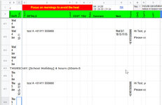
Dates are in B, times are in C, ID (a phone number) is in L

This works for for a next single applintment...
=if(L5="" , "",IFNA(LEFT(text(INDEX(B6:B$1559,MATCH(L5,L6:L$1559,0)),"dddd"), 3),"") & IFNA(text(INDEX(B6:B$1559,MATCH(L5,L6:L$1559,0)), " d/m"),"") &
" at " &
IFNA(INDEX(C6:C$1559,MATCH(L5,L6:L$1559,0)),"") )

giving:
Wed 14/9 at 8:45-10:45

Is there a way to get a list of all future appointments?
 

Attachments

  • Test time.jpg
    Test time.jpg
    141.7 KB · Views: 25

Excel Facts

Using Function Arguments with nested formulas
If writing INDEX in Func. Arguments, type MATCH(. Use the mouse to click inside MATCH in the formula bar. Dialog switches to MATCH.
Do you mean that in K617 you want the formula to look down the list until it hits the next set of B:C cells after row 618?
 
Upvote 0
Yeah.
Or looking a it another way, K612 would list B617:C617 as it does, and any further appointments with that phone number.
So if there was say, a Saturday 7 booking at 10:00-11:00, K612 would read:

Wed 5/1
10:15-11:15

Sat 7/1
10:00-11:00

Horizontal space is limited, so the pic shows how it is now, else I'd have each entry to its own line, like in sample above
 
Upvote 0
K612 would list B617:C617 as it does, and any further appointments with that phone number.
So if there was say, a Saturday 7 booking at 10:00-11:00, K612 would read:

Wed 5/1
10:15-11:15

Sat 7/1
10:00-11:00

So you're asking for essentially a forward looking Vlookup that returns all matching results.
What you're asking can be done with TEXTJOIN.


Excel Formula:
=TEXTJOIN(CHAR(10)&CHAR(10),TRUE,IF(L4:L42=L4,(TEXT(B4:B42,"DD/MM/YY")&CHAR(10)&TEXT(C4:C42,"H:MM")),""))

Explanation
TEXTJOIN does the Vlookup.
CHAR(10) gives you new lines inside a cell, we delimit the list returned by text join with two new lines. Each entry in the list is a concatenation of the column B and C arrays with a new line between them.
The column B and C arrays will show up as numbers when concatenated. They are converted to TEXT first in a format of our choosing (DD/MM/YYYY, H:MM) before we concatenate.

1671577418256.png
 
Upvote 1
Solution
That's fantastic! Thank you.
Um, but I'm using Sheets and Sheets doesn't like TEXTJOIN.
(My bad, I posted in 'Other' but forgot to specify Sheets, sorry about that)

Can you whizz up a solution for sheets?
 

Attachments

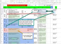
  • Mapping-bookings.jpg
    Mapping-bookings.jpg
    131.6 KB · Views: 6
Upvote 0
Google sheets will be able to use the formula from my brief 5 minute search provided you wrap the whole thing in =ARRAYFORMULA()

and yeah apologies I've stumbled into the wrong forum. I usually just look for unanswered excel questions.
 
Upvote 1

Forum statistics

Threads
1,223,227
Messages
6,170,848
Members
452,361
Latest member
d3ad3y3

We've detected that you are using an adblocker.

We have a great community of people providing Excel help here, but the hosting costs are enormous. You can help keep this site running by allowing ads on MrExcel.com.
Allow Ads at MrExcel

Which adblocker are you using?

Disable AdBlock

Follow these easy steps to disable AdBlock

1)Click on the icon in the browser’s toolbar.
2)Click on the icon in the browser’s toolbar.
2)Click on the "Pause on this site" option.
Go back

Disable AdBlock Plus

Follow these easy steps to disable AdBlock Plus

1)Click on the icon in the browser’s toolbar.
2)Click on the toggle to disable it for "mrexcel.com".
Go back

Disable uBlock Origin

Follow these easy steps to disable uBlock Origin

1)Click on the icon in the browser’s toolbar.
2)Click on the "Power" button.
3)Click on the "Refresh" button.
Go back

Disable uBlock

Follow these easy steps to disable uBlock

1)Click on the icon in the browser’s toolbar.
2)Click on the "Power" button.
3)Click on the "Refresh" button.
Go back
Back
Top