how to Find the cell position of a Duplicated smallest values in a data set ?

Anjelo

New Member
Joined
Apr 2, 2021
Messages
4
Office Version
  1. 2019
Platform
  1. Windows
Hello every one ..
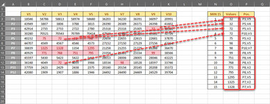
If i have a data set like this one in the attached picture ,
Is there any way to find the positions as a result in column "P" by finding the the smallest values in column "O".
Notes that there are a duplicated smallest values in different positions in the data set.
 

Attachments

  • Wanted.jpg
    Wanted.jpg
    226.2 KB · Views: 15

Excel Facts

How to fill five years of quarters?
Type 1Q-2023 in a cell. Grab the fill handle and drag down or right. After 4Q-2023, Excel will jump to 1Q-2024. Dash can be any character.
Removed, as there was an error.
 
Last edited:
Upvote 0
Hi & welcome to MrExcel.
How about
+Fluff 1.xlsm
ABCDEFGHIJKLMNOPQ
1
2V1V2V3V4V5V6V7V8V9V10
3P1125105628415511562311938192910601148148P8V9
4P215917575401638195231713561441103952252P2V10
5P3177414701441333299148625911341171119352P6V1
6P47467651178171363123646018246871048466P11V6
7P565817272871154115877014847091581888599P12V10
8P652117176318731391626115511421177916117P3V9
9P7111216210606281214132614943672111727117P4V3
10P81923132722213571033413371215488458117P6V2
11P9157240119107383916021594430101415529117P6V9
12P1016971263251901231551176118131851157810119P9V3
13P11170780994913731878661735249104859311125P1V1
14P121572379538114512693555951411599912126P10V2
1513126P12V5
1614135P8V4
1715139P6V5
Main
Cell Formulas
RangeFormula
O3:O17O3=SMALL($B$3:$K$14,N3)
P3:P17P3=INDEX($A$3:$A$14,INT((AGGREGATE(15,6,ROW($1:$120)/(FILTERXML("<k><m>"&TEXTJOIN("</m><m>",,$B$3:$K$14)&"</m></k>","//m")=O3),COUNTIFS(O$3:O3,O3))-1)/10)+1)
Q3:Q17Q3=INDEX($B$2:$K$2,MOD(AGGREGATE(15,6,ROW($1:$120)/(FILTERXML("<k><m>"&TEXTJOIN("</m><m>",,$B$3:$K$14)&"</m></k>","//m")=O3),COUNTIFS(O$3:O3,O3))-1,10)+1)
thank you so much ... it looks exactly what i am looking for ,, but i got an issues that the calculation is not correct like in the attached picture
thank you again

Wanted 5.png
 
Upvote 0
For that range you would need to use
+Fluff 1.xlsm
ABCDEFGHIJKLMNOPQRS
1
2
3V1V2V3V4V5V6V7V8V9V10V11V12
4P11251056284155115623119381929106011481108875127P19V11
5P2159175754016381952317135614411039521222161230P18V6
6P31774147014413332991486259113411711191288333348P8V9
7P474676511781713631236460182468710484141704452P2V10
8P5658172728711541158770148470915818884981133552P6V1
9P652117176318731391626115511421177916951943655P17V7
10P7111216210606281214132614943672111721406110761P9V11
11P819231327222135710334133712154884517791467866P11V6
12P9157240119107383916021594430101415526197975P13V4
13P1016971263251901231551176118131851157875619151089P20V4
14P111707809949137318786617352491048593198015391192P20V7
15P12157237953811451269355595141159998322091297P9V12
16P1376668142175494819188518591521108453018561399P12V10
17P141911123439456616661277455912201176195367314110P7V12
18P151930123672511948441688697681119740383168615117P3V9
19P165444758871948105737743814686295871211955
20P171303164319481860167317195518472331477677620
21P1817851501137218219743011751407184721517721883
22P191276552284185618518411969388157213271211
23P20154758157689154723492117211141919250317
Main
Cell Formulas
RangeFormula
Q4:Q18Q4=SMALL($C$4:$N$23,P4)
R4:R18R4=INDEX($B$4:$B$23,INT((AGGREGATE(15,6,ROW($1:$240)/(FILTERXML("<k><m>"&TEXTJOIN("</m><m>",,$C$4:$N$23)&"</m></k>","//m")=Q4),COUNTIFS(Q$4:Q4,Q4))-1)/12)+1)
S4:S18S4=INDEX($C$3:$N$3,MOD(AGGREGATE(15,6,ROW($1:$240)/(FILTERXML("<k><m>"&TEXTJOIN("</m><m>",,$C$4:$N$23)&"</m></k>","//m")=Q4),COUNTIFS(Q$4:Q4,Q4))-1,12)+1)
 
Upvote 0
Solution
For reference with this
Rich (BB code):
=INDEX($B$4:$B$23,INT((AGGREGATE(15,6,ROW($1:$240)/(FILTERXML("<k><m>"&TEXTJOIN("</m><m>",,$C$4:$N$23)&"</m></k>","//m")=Q4),COUNTIFS(Q$4:Q4,Q4))-1)/12)+1)
The part in blue needs to be the total number of cells being looked at. C4:N23 = 240 cells.
The part in Red is the number of columns being looked at. C4:N4 =12 columns
 
Upvote 0
For that range you would need to use
+Fluff 1.xlsm
ABCDEFGHIJKLMNOPQRS
1
2
3V1V2V3V4V5V6V7V8V9V10V11V12
4P11251056284155115623119381929106011481108875127P19V11
5P2159175754016381952317135614411039521222161230P18V6
6P31774147014413332991486259113411711191288333348P8V9
7P474676511781713631236460182468710484141704452P2V10
8P5658172728711541158770148470915818884981133552P6V1
9P652117176318731391626115511421177916951943655P17V7
10P7111216210606281214132614943672111721406110761P9V11
11P819231327222135710334133712154884517791467866P11V6
12P9157240119107383916021594430101415526197975P13V4
13P1016971263251901231551176118131851157875619151089P20V4
14P111707809949137318786617352491048593198015391192P20V7
15P12157237953811451269355595141159998322091297P9V12
16P1376668142175494819188518591521108453018561399P12V10
17P141911123439456616661277455912201176195367314110P7V12
18P151930123672511948441688697681119740383168615117P3V9
19P165444758871948105737743814686295871211955
20P171303164319481860167317195518472331477677620
21P1817851501137218219743011751407184721517721883
22P191276552284185618518411969388157213271211
23P20154758157689154723492117211141919250317
Main
Cell Formulas
RangeFormula
Q4:Q18Q4=SMALL($C$4:$N$23,P4)
R4:R18R4=INDEX($B$4:$B$23,INT((AGGREGATE(15,6,ROW($1:$240)/(FILTERXML("<k><m>"&TEXTJOIN("</m><m>",,$C$4:$N$23)&"</m></k>","//m")=Q4),COUNTIFS(Q$4:Q4,Q4))-1)/12)+1)
S4:S18S4=INDEX($C$3:$N$3,MOD(AGGREGATE(15,6,ROW($1:$240)/(FILTERXML("<k><m>"&TEXTJOIN("</m><m>",,$C$4:$N$23)&"</m></k>","//m")=Q4),COUNTIFS(Q$4:Q4,Q4))-1,12)+1)
Thank you soooooooooooo much ... Now everything is 100% correct ,, :love::love::love::love:
 
Upvote 0
You're welcome & thanks for the feedback.
 
Upvote 0
If you're interested, 2simpler formulae
+Fluff 1.xlsm
ABCDEFGHIJKLMNOPQTU
1
2
3V1V2V3V4V5V6V7V8V9V10V11V12
4P11251056284155115623119381929106011481108875127P19V11
5P215917575401638195231713561441103952122261230P18V6
6P31774147014413332991486259113411711191288333348P8V9
7P474676511781713631236460182468710484141704452P2V10
8P565817272871154115877014847091581888611133552P6V1
9P652117176318731391626115511421177916951943655P17V7
10P7111216210606281214132614943672111721406110761P2V12
11P819231327222135710334133712154884517791467861P5V11
12P96116111910736116021594430101415526197961P9V1
13P1016971263251901231551176118131851157875619151061P9V5
14P111707809949137318786617352491048593198015391161P9V11
15P12157237953811451269355595141159998322091266P11V6
16P1376668142175494819188518591521108453018561375P13V4
17P14191112343945661666127745591220117619536731489P20V4
18P15193012367251194844168869768111974038316861592P20V7
19P165444758871948105737743814686295871211955
20P171303164319481860167317195518472331477677620
21P1817851501137218219743011751407184721517721883
22P191276552284185618518411969388157213271211
23P20154758157689154723492117211141919250317
Main
Cell Formulas
RangeFormula
Q4:Q18Q4=SMALL($C$4:$N$23,P4)
T4:T18T4=INDEX($B$4:$B$23,AGGREGATE(15,6,(ROW($B$4:$B$23)-ROW($B$4)+1)/($C$4:$N$23=Q4),COUNTIFS(Q$4:Q4,Q4)))
U4:U18U4=INDEX($C$3:$N$3,AGGREGATE(15,6,(COLUMN($C$3:$N$3)-COLUMN($C$3)+1)/($C$4:$N$23=Q4)/($B$4:$B$23=R4),COUNTIFS(Q$4:Q4,Q4,R$4:R4,R4)))
thank you soooo much this one much more efficient ... ammazing (y)(y)(y)(y)(y)(y)(y)(y)(y)(y)
 
Upvote 0

Forum statistics

Threads
1,224,937
Messages
6,181,858
Members
453,068
Latest member
DCD1872

We've detected that you are using an adblocker.

We have a great community of people providing Excel help here, but the hosting costs are enormous. You can help keep this site running by allowing ads on MrExcel.com.
Allow Ads at MrExcel

Which adblocker are you using?

Disable AdBlock

Follow these easy steps to disable AdBlock

1)Click on the icon in the browser’s toolbar.
2)Click on the icon in the browser’s toolbar.
2)Click on the "Pause on this site" option.
Go back

Disable AdBlock Plus

Follow these easy steps to disable AdBlock Plus

1)Click on the icon in the browser’s toolbar.
2)Click on the toggle to disable it for "mrexcel.com".
Go back

Disable uBlock Origin

Follow these easy steps to disable uBlock Origin

1)Click on the icon in the browser’s toolbar.
2)Click on the "Power" button.
3)Click on the "Refresh" button.
Go back

Disable uBlock

Follow these easy steps to disable uBlock

1)Click on the icon in the browser’s toolbar.
2)Click on the "Power" button.
3)Click on the "Refresh" button.
Go back
Back
Top