How can I calculate targeted count cumulatively

MosMon

New Member
Joined
Sep 25, 2014
Messages
3
Office Version
  1. 2019
  2. 2016
Platform
  1. Windows
Greetings,

I have sales numbers for each Distributor. we have a new policy that Distributors will get free units from the mother company if they meet the target. But the problem is this free unit should be calculated based on cumulative sales and counted from the maximum target. Thus, seeking the expert help, please.

An example is given below:
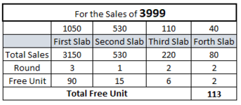
Assume that the distributor sales 3999 unit in a month. thus, free unit calculation is

=1050*3=3150 which will be equivalent to 30*3
Rest, 849, which will be under 530 sales quantity. And free unit is 15
Rest, 319, Which will be under 110 sales quantity. And free unit is 3*2
Rest, 99, Which will be under 40 sales quantity. And free unit is 2*1

So Finally total free unit is: 30*3+15*1+3*2+2*1=113

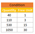
Condition
Sales QuantityFree Unit
401
1103
53015
105030

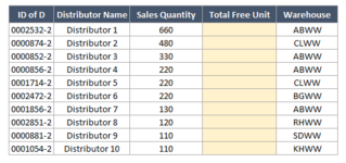
ID of DDistributor NameSales QuantityTotal Free UnitWarehouse
0002532-2Distributor 1660ABWW
0000874-2Distributor 2480CLWW
0000852-2Distributor 3330ABWW
0000856-2Distributor 4220ABWW
0001714-2Distributor 5220CLWW
0002472-2Distributor 6220BGWW
0001856-2Distributor 7130ABWW
0002851-2Distributor 8120RHWW
0000881-2Distributor 9110SDWW
0001054-2Distributor 10110KHWW

For the Sales of 3999
105053011040
First SlabSecond SlabThird SlabForth Slab
Total Sales315053022080
Round3122
Free Unit901562
Total Free Unit113
 

Attachments

  • MREXCEL1.png
    MREXCEL1.png
    17.3 KB · Views: 4
  • MREXCEL2.png
    MREXCEL2.png
    2.8 KB · Views: 4
  • MREXCEL3.png
    MREXCEL3.png
    6.4 KB · Views: 5

Excel Facts

Return population for a City
If you have a list of cities in A2:A100, use Data, Geography. Then =A2.Population and copy down.
Here is one approach involving setting up some helper cells to the right of your table (can hide them if deisred). You don't really need the last helper column, but you do need the array starting with the Sales Qty (which has been copied over to column G) and the results of the next three MOD operations. I thought this layout made more sense as the result of the MOD operation resides at the coordinates of its arguments.
Book1
CDEFGHIJK
1Sales QtyFree UnitsQty \ Slabs105053011040
2399911339998493199919
3660186606601302020
4567816156784284289818
548013480480480400
699992859999549191919
Sheet2
Cell Formulas
RangeFormula
G2:G6G2=C2
H2:K6H2=MOD(G2,H$1)
D2:D6D2=SUMPRODUCT(QUOTIENT(+G2:J2,{1050,530,110,40}),{30,15,3,1})
 
Last edited:
Upvote 0
Greetings Mr. KRice,

I'm extremely thankful to you to get the solution. I can do a similar type of solution with the combination of Lookup, Vlookup, and IF. where 8 columns are required. Is it possible to find out the answer using a single column? Seeking your suggestion, please.
I'm really grateful to you again. Thank you
 
Upvote 0
What version of Excel are you using? You should update your account profile with that information as some solution options depend on the version. I ask about the version because somehow you need to form an array of the remainders after each slab is evaluated, so recursion is necessary...the input for the next step depends on the result from the last step. If you have Excel 365, this may be doable in a single formula, but if you don't have 365, I don't see a way to do it without some helper cells. My approach above could be reduced to four columns wide as shown here, and those columns could be hidden. And as an example of doing this with a single formula in Excel 365, you could do something like I'm showing in D19:D23 using a LET function with SEQUENCE to construct the array...there may be a more elegant way to do that rather than nesting 4 IF statements, but it works!
MrExcel_20220607.xlsx
CDEFGHI
10Sales QtyFree Units
113999113399984931999
126601866066013020
135678161567842842898
144801348048048040
15999928599995491919
16
17single formula
18Sales QtyFree Units
193999113
2066018
215678161
2248013
239999285
Sheet2
Cell Formulas
RangeFormula
F11:F15F11=C11
G11:G15G11=MOD(F11,1050)
H11:H15H11=MOD(G11,530)
I11:I15I11=MOD(H11,110)
D11:D15D11=SUMPRODUCT(QUOTIENT(+F11:I11,{1050,530,110,40}),{30,15,3,1})
D19:D23D19=SUMPRODUCT(QUOTIENT(LET(v,$C19,s,SEQUENCE(,4),IF(s=1,v,IF(s=2,MOD(v,1050),IF(s=3,MOD(MOD(v,1050),530),IF(s=4,MOD(MOD(MOD(v,1050),530),110)))))),{1050,530,110,40}),{30,15,3,1})
 
Upvote 0
Greetings Mr. KRice,

you're awesome.

Thanks for your suggestion. I have updated my office version which is 2019 and 2016 (Two different laptop).
I have tried your formula but not working. And I have tried many combinations based on your pattern but failed.

Thus, seeking your expert support, please
 
Upvote 0
The single formula version will not work on versions earlier than 365, as the single formula uses functions (LET and SEQUENCE) and array forming techniques that aren't available/possible in 2016 or 2019. The 4-column helper version should work, I think. One thing to watch for: the QUOTIENT function needs that unary plus operator to allow the function to accept the range as an array...so it should be as shown QUOTIENT(+...

If that doesn't help, please post other details and the formula that you are using.
 
Upvote 0
Try this
ConditionColumnD
Sales QuantityFree Unit
40​
1​
110​
3​
530​
15​
1050​
30​
ID of DDistributor NameSales QuantityTotal Free UnitWarehouseRow8
0002532-2Distributor 1
1660​
47ABWWRow9
0000874-2Distributor 2
3480​
99CLWWRow10
0000852-2Distributor 3
830​
23ABWWRow11
0000856-2Distributor 4
220​
6ABWWRow12
0001714-2Distributor 5
220​
6CLWWRow13
0002472-2Distributor 6
202​
5BGWWRow14
0001856-2Distributor 7
130​
3ABWWRow15
0002851-2Distributor 8
120​
3RHWWRow16
0000881-2Distributor 9
110​
3SDWWRow17
0001054-2Distributor 10
90​
2KHWWRow18

In D9 copied down
Excel Formula:
=$B$6*INT(C9/$A$6)+$B$5*(INT(MOD(C9,$A$6)/$A$5))+$B$4*(INT(MOD(MOD(C9,$A$6),$A$5)/$A$4))+$B$3*INT(MOD(MOD(MOD(C9,$A$6),$A$5),$A$4)/$A$3)
 
Upvote 0
As a variation on the nested MOD's with QUOTIENT or INT functions, you could eliminate the helper table altogether and hardwire the slab thresholds and free unit values directly in for a single formula approach with no other support cells needed:
MrExcel_20220607.xlsx
CD
30Sales QtyFree Units
313999113
3266018
335678161
3448013
359999285
Sheet2
Cell Formulas
RangeFormula
D31:D35D31=30*INT(C31/1050)+15*(INT(MOD(C31,1050)/530))+3*(INT(MOD(MOD(C31,1050),530)/110))+1*INT(MOD(MOD(MOD(C31,1050),530),110)/40)
 
Upvote 0
This slightly tighter version eliminates some unneeded characters in the formula (this is from cell D31 and refers to Sales Quantity in C31):
Excel Formula:
=30*INT(C31/1050)+15*INT(MOD(C31,1050)/530)+3*INT(MOD(MOD(C31,1050),530)/110)+INT(MOD(MOD(MOD(C31,1050),530),110)/40)
 
Upvote 0

Forum statistics

Threads
1,224,564
Messages
6,179,543
Members
452,924
Latest member
JackiG

We've detected that you are using an adblocker.

We have a great community of people providing Excel help here, but the hosting costs are enormous. You can help keep this site running by allowing ads on MrExcel.com.
Allow Ads at MrExcel

Which adblocker are you using?

Disable AdBlock

Follow these easy steps to disable AdBlock

1)Click on the icon in the browser’s toolbar.
2)Click on the icon in the browser’s toolbar.
2)Click on the "Pause on this site" option.
Go back

Disable AdBlock Plus

Follow these easy steps to disable AdBlock Plus

1)Click on the icon in the browser’s toolbar.
2)Click on the toggle to disable it for "mrexcel.com".
Go back

Disable uBlock Origin

Follow these easy steps to disable uBlock Origin

1)Click on the icon in the browser’s toolbar.
2)Click on the "Power" button.
3)Click on the "Refresh" button.
Go back

Disable uBlock

Follow these easy steps to disable uBlock

1)Click on the icon in the browser’s toolbar.
2)Click on the "Power" button.
3)Click on the "Refresh" button.
Go back
Back
Top