How can I auto-copy a cell formula reference to each row?

srob93

New Member
Joined
Dec 28, 2020
Messages
14
Platform
  1. Web
Hello,

I am somewhat of a novice to excel/gsheet and really need some help.

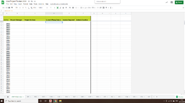
Currently creating a '2021 job tracker' and need the 'Overview' page to sync to certain cells in each individual job tracker.

See attached.

Cell D3 =MASTER!C24

I then need Cell D4 to say =001!C24, Cell D5 to say =002!C24, Cell D6 to say =003!C24... then 004, 005, 006 and so on.

Is there a way to do this automatically without having to update each individual formula?

Thank you in advance!! :)
 

Attachments

  • gsheet query.png
    gsheet query.png
    134.3 KB · Views: 14

Excel Facts

Did you know Excel offers Filter by Selection?
Add the AutoFilter icon to the Quick Access Toolbar. Select a cell containing Apple, click AutoFilter, and you will get all rows with Apple
I am not sure if it is exactly the same in Google Sheets, but in Excel, you can place the following formula in cell D4 and copy across (D5, D6, ...), and it will return what you want:
Excel Formula:
=INDIRECT(TEXT(COLUMN()-3,"000")&"!C24")
 
Upvote 0
I am not sure if it is exactly the same in Google Sheets, but in Excel, you can place the following formula in cell D4 and copy across (D5, D6, ...), and it will return what you want:
Excel Formula:
=INDIRECT(TEXT(COLUMN()-3,"000")&"!C24")
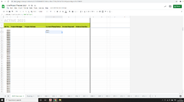
Hi Joe4 - thanks so much for your reply.

See attached.

That is so so close to what I am after. It has worked perfectly for cell D4, but when I copy the formula in to D5 it still links to the same reference as cell D4. I need Cell D5 to link to tab 002, and cell D6 to link to tab 003, and so on.

Any ideas?
 

Attachments

  • gsheet query #4.png
    gsheet query #4.png
    139.8 KB · Views: 22
Upvote 0
Do you have to do someting in Google Docs to make it recalc?
Try entering this formula in E4 and copy to E5 and E6, and see what it returns in each cell:
Excel Formula:
=TEXT(COLUMN()-3,"000")&"!C24"
 
Upvote 0
Do you have to do someting in Google Docs to make it recalc?
Try entering this formula in E4 and copy to E5 and E6, and see what it returns in each cell:
Excel Formula:
=TEXT(COLUMN()-3,"000")&"!C24"

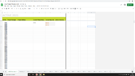
Have done... see attached.

What do you think?
 

Attachments

  • gsheet query #6.png
    gsheet query #6.png
    138.1 KB · Views: 13
Upvote 0
Ha! I went the wrong way in my formula (I went across instead of down).
You want to use ROW() instead of COLUMN(), i.e.
Excel Formula:
=INDIRECT(TEXT(ROW()-3,"000")&"!C24")
Sorry about that.
 
Upvote 0
Solution
Ha! I went the wrong way in my formula (I went across instead of down).
You want to use ROW() instead of COLUMN(), i.e.
Excel Formula:
=INDIRECT(TEXT(ROW()-3,"000")&"!C24")
Sorry about that.

YES!! ? ? ? ? ? ?

Thank you so much - you have just made my like 10000 times easier!!!
 
Upvote 0
You are welcome! Glad I was able to help!

The secret is to build the reference dynamically. However, when you do that, it will return a string, not a range reference.
To convert it to a range reference, you wrap the formula in "INDIRECT".

The other key is that using the ROW() and.or COLUMNS() functions returns the current row/column that the formula is in.
That is how we get the reference to increase by one row as we move down rows.
You can see this easily if you enter the formula =ROW() into any cell, and then copy it down.
 
Upvote 0

Forum statistics

Threads
1,223,630
Messages
6,173,454
Members
452,514
Latest member
cjkelly15

We've detected that you are using an adblocker.

We have a great community of people providing Excel help here, but the hosting costs are enormous. You can help keep this site running by allowing ads on MrExcel.com.
Allow Ads at MrExcel

Which adblocker are you using?

Disable AdBlock

Follow these easy steps to disable AdBlock

1)Click on the icon in the browser’s toolbar.
2)Click on the icon in the browser’s toolbar.
2)Click on the "Pause on this site" option.
Go back

Disable AdBlock Plus

Follow these easy steps to disable AdBlock Plus

1)Click on the icon in the browser’s toolbar.
2)Click on the toggle to disable it for "mrexcel.com".
Go back

Disable uBlock Origin

Follow these easy steps to disable uBlock Origin

1)Click on the icon in the browser’s toolbar.
2)Click on the "Power" button.
3)Click on the "Refresh" button.
Go back

Disable uBlock

Follow these easy steps to disable uBlock

1)Click on the icon in the browser’s toolbar.
2)Click on the "Power" button.
3)Click on the "Refresh" button.
Go back
Back
Top