Help with sequential numbering

[quickflip]

Hi there everyone

I'm new here and come here to find some help about a problem that seems easy to solve but i can't do it. It has 2 parts this problem

The first one is i need a solution to automatically fill in the serial number column (column C) sequentialy and acordding to column A (example given). I tried a solution with count ifs but didnt work as expected

The other one is a solution to the ID. I want to create a highlight formula that highlights only the Unique ID's values that are doubled on that column and makes an exception on the "NOT FOUND" ones (since there are a lot of them because they come from a VLOOKUP)

Kind Regards

111.xlsx
	A	B	C	D
4	VARIANT	Prod. ID	SERIAL NUMBER	ID
5	A	1	SA-1	Unique ID
6	B	2	SB-1	Unique ID
7	A	3	SA-2	Unique ID
8	A	4	SA-3	Unique ID
9	C	5	SC-1	Unique ID
10	C	6	SC-2	Unique ID
11	C	7	SC-3	Unique ID
12	C	8	SC-4	NOT FOUND
13	D	9	SD-1	Unique ID
14	A	10	SA-4	Unique ID
15	D	11	SD-2	NOT FOUND
Sheet1

 

[Joe4]

Welcome to the Board!

Assuming that your data is in column A, and starts on row 2 (title row in row 1), then here is a formula for your Serial Number you can place in row 2 and copy down for all rows:

="S" & A2 & "-" & COUNTIF($A$2:$A2,$A2)

I am not sure I follow your second question.
Can you try explaining that again?
Is that "ID" column already populated, or do you need a formula for it?

 

[quickflip]

Hello there.

Thanks for the reply. Ill try the first solution you gave me

So the unique ID comes automatically from another worksheet as I said and I want to create a highlight conditional formatting rule that only highlights the unique ids that could be duplicate and leaves the duplicates not found on the side, without formatting.

Kind Regards.

 

[Joe4]

So the unique ID comes automatically from another worksheet as I said and I want to create a highlight conditional formatting rule that only highlights the unique ids that could be duplicate and leaves the duplicates not found on the side, without formatting.

I guess I do not understand how to determine which ones "may be duplicates".
Can you explain that logic a little more clearly?
And tell us in your example, which ones should be highlighted by Conditional Formatting?

 

[quickflip]

Also, the solution is not quite that, for the first question

More or less is like this that I want

The variant type has a data validation list with 4 variants (111111,222222...)

111.xlsx
	A	B	C	D
2	111111	1	SA-1	Unique ID
3	222222	2	SB-1	Unique ID
4	111111	3	SA-2	Unique ID
5	111111	4	SA-3	Unique ID
6	333333	5	SC-1	Unique ID
7	333333	6	SC-2	Unique ID
8	333333	7	SC-3	Unique ID
9	333333	8	SC-4	NOT FOUND
10	444444	9	SD-1	Unique ID
11	111111	10	SA-4	Unique ID
12	444444	11	SD-2	NOT FOUND
Sheet1

 

[quickflip]

Sure I can explain.
Imagine that i insert on column B2 and B3 two diferent values. On D column, with a VLOOKUP, its going to give me those unique ID's for each cell. But i want to make sure that there is no duplicate id's that come from that vlookup so i want to highlight them. So if the vlookup value = NOT FOUND or ERROR, ignore the formatting rule. else, try to find the values that are duplicate on column D

 

[Joe4]

Also, the solution is not quite that, for the first question

More or less is like this that I want

The variant type has a data validation list with 4 variants (111111,222222...)

111.xlsx
	A	B	C	D
2	111111	1	SA-1	Unique ID
3	222222	2	SB-1	Unique ID
4	111111	3	SA-2	Unique ID
5	111111	4	SA-3	Unique ID
6	333333	5	SC-1	Unique ID
7	333333	6	SC-2	Unique ID
8	333333	7	SC-3	Unique ID
9	333333	8	SC-4	NOT FOUND
10	444444	9	SD-1	Unique ID
11	111111	10	SA-4	Unique ID
12	444444	11	SD-2	NOT FOUND
Sheet1

That changes the questions quite a bit, and shows how important it is to accurately depict your examples, as it looked like the SERIAL NUMBER field used the VARIANT value. The fact that it does not changes things quite a bit.

How many possible different VARIANT values might you have?
If more than 26, what happens after you get to "SZ..."?
What would the 27th SERIAL NUMBER value look like?

 

[quickflip]

That changes the questions quite a bit, and shows how important it is to accurately depict your examples, as it looked like the SERIAL NUMBER field used the VARIANT value. The fact that it does not changes things quite a bit.

How many possible different VARIANT values might you have?
If more than 26, what happens after you get to "SZ..."?
What would the 27th SERIAL NUMBER value look like?

I have 4 variants (1111,2222,3333,4444) that i want to assemble at a assembly line. after that, i want to give them a serial number based on their status. The total number of variants (parts) would be a 1000 (1000 rows)

Kind regards

 

[Joe4]

Sure I can explain.
Imagine that i insert on column B2 and B3 two diferent values. On D column, with a VLOOKUP, its going to give me those unique ID's for each cell. But i want to make sure that there is no duplicate id's that come from that vlookup so i want to highlight them. So if the vlookup value = NOT FOUND or ERROR, ignore the formatting rule. else, try to find the values that are duplicate on column D

I am sorry, I am just not getting what you are saying.
Please try to walk through the data example you posted and explain for those particular records which ones should be highlighted and why.

I have 4 variants (1111,2222,3333,4444) that i want to assemble at a assembly line. after that, i want to give them a serial number based on their status. The total number of variants (parts) would be a 1000 (1000 rows)

OK, try this then:

="S" & LOOKUP(A2,{111111,222222,333333,444444},{"A","B","C","D"}) & "-" & COUNTIF($A$2:$A2,$A2)

 

[quickflip]

Hi there

I think that that might work, ill try it now

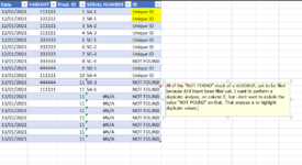
Regarding the other question, ill make an example

Kind regards