Group by IDs and calculate

[OCM]

Greetings,

Using Excel 365 and given the following in the attached sample:

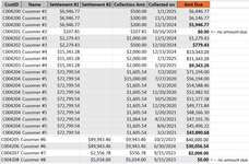
Amount due = Settlement #1 – Collection amount (if Settlement #1 is not blank)
Amount due = Settlement #2 – Collection amount (if Settlement #1 is blank)
If Amount due = 0, then display “no amount due”

I would like to create a new column to calculate the itemized collection payments/amt. and display the amount due per CustID at the bottom. Please see the expected result in the attached sample.



TIA

Regards,

 

[hagia_sofia]

Hello, as I am not entirely sure what is the expected output, could you please share with us here whether it is what is depiced in the last column or whether is a list of unique IDs with the corresponding last (bold) amount?

 

[OCM]

Thanks for the reply post.

The expected result is the last column which for this example I manually did the calculation and show the amount due at the bottom. Since my data consists of over 2000 records, I though a pivot table and/or applying formula to the logic will be a way to go.



TIA

Regards,

 

[hagia_sofia]

Many thanks for the clarification. So, maybe something like:

=LET(
c,IF((B1=B2)=FALSE,(C2&D2)-E2,G1-E2),
IF(c=0,"no amount due",c))

Please note that the formula uses customer name instead of customer ID as it corresponds with your calculation as two different customer IDs (C004205 and C004206) are related to a single customer (#6).

 

[Peter_SSs]

Same suggestion, just a little more compact.

25 03 03.xlsm
	B	C	D	E		G
1	Name	S #1	S #2	Amt		Amt Due
2	Cust #1	7,000.00		500.00		6,500.00
3	Cust #1	7,000.00		300.00		6,200.00
4	Cust #1	7,000.00		200.00		6,000.00
5	Cust #2	123.00		123.00		no amount due
6	Cust #3	2,000.00		1,000.00		1,000.00
7	Cust #3	2,000.00		500.00		500.00
8	Cust #4	15,000.00		2,000.00		13,000.00
9	Cust #4	15,000.00		2,000.00		11,000.00
10	Cust #4	15,000.00		2,000.00		9,000.00
11	Cust #5	72,800.00		1,605.00		71,195.00
12	Cust #5	72,800.00		15,000.00		56,195.00
13	Cust #5	72,800.00		1,605.54		54,589.46
14	Cust #5	72,800.00		1,605.54		52,983.92
15	Cust #5	72,800.00		1,605.54		51,378.38
16	Cust #5	72,800.00		1,605.54		49,772.84
17	Cust #5	72,800.00		1,605.54		48,167.30
18	Cust #5	72,800.00		1,605.54		46,561.76
19	Cust #5	72,800.00		1,605.54		44,956.22
20	Cust #5	72,800.00		1,605.54		43,350.68
21	Cust #6		50,000.00	9,900.00		40,100.00
22	Cust #6		50,000.00	9,900.00		30,200.00
23	Cust #7		2,500.00	500.00		2,000.00
24	Cust #8		5,000.00	5,000.00		no amount due
Amt Due

Cell Formulas
Range	Formula
G2:G24	G2	=LET(c,IF(B1=B2,G1,C2&D2)-E2,IF(c,c,"no amount due"))

 

[Peter_SSs]

Or if you are just looking for the summary (final row for each customer)

25 03 03.xlsm
	B	C	D	E			H	I	J
1	Name	S #1	S #2	Amt				Name	Amt Due
2	Cust #1	7,000.00		500.00				Cust #1	6,000.00
3	Cust #1	7,000.00		300.00				Cust #2	no amount due
4	Cust #1	7,000.00		200.00				Cust #3	500.00
5	Cust #2	123.00		123.00				Cust #4	9,000.00
6	Cust #3	2,000.00		1,000.00				Cust #5	43,350.68
7	Cust #3	2,000.00		500.00				Cust #6	30,200.00
8	Cust #4	15,000.00		2,000.00				Cust #7	2,000.00
9	Cust #4	15,000.00		2,000.00				Cust #8	no amount due
10	Cust #4	15,000.00		2,000.00
11	Cust #5	72,800.00		1,605.00
12	Cust #5	72,800.00		15,000.00
13	Cust #5	72,800.00		1,605.54
14	Cust #5	72,800.00		1,605.54
15	Cust #5	72,800.00		1,605.54
16	Cust #5	72,800.00		1,605.54
17	Cust #5	72,800.00		1,605.54
18	Cust #5	72,800.00		1,605.54
19	Cust #5	72,800.00		1,605.54
20	Cust #5	72,800.00		1,605.54
21	Cust #6		50,000.00	9,900.00
22	Cust #6		50,000.00	9,900.00
23	Cust #7		2,500.00	500.00
24	Cust #8		5,000.00	5,000.00
Amt Due

Cell Formulas
Range	Formula
I2:J9	I2	=LET(b,B2:B24,u,UNIQUE(b),HSTACK(u,BYROW(u,LAMBDA(r,LET(c,TAKE(FILTER(C2:C24&D2:D24,b=r),1)-SUMIFS(E2:E24,b,r),IF(c,c,"no amount due"))))))
Dynamic array formulas.

 

[RoryA]

A gentle reminder:

Cross-posting (posting the same question in more than one forum) is not against our rules, but the method of doing so is covered by #13 of the Forum Rules.

Be sure to follow & read the link at the end of the rule too!

Cross posted at:

UtterAccess.com

www.utteraccess.com

There is no need to repeat the link(s) provided above but if you have posted the question at other places, please provide links to those as well.

If you do cross-post in the future and also provide links, then there shouldn’t be a problem.

 

[OCM]

Hagia_Sofia,

Thanks for the feedback. I’m glad you caught this. The formula should use customer IDs instead of customer name as the same customer can have multiple IDs at a different time. That is why I banded/grouped by the customer ID on my sample.

As a result, the amount due for both Customer #6s (C004205 & C004206 should be $40,000. I incorrectly put $30,056.54 for C004206 when I manually populated the amount due (column ‘g’). My apologies.



Peter_SSs, I applied both your suggestions and got the expected results in both. I even explored, altered your formula to =LET(c,IF(B1=B2,G1,C2&D2)-E2,IF(c,c,0)) if I decide to show $0.00 in the future.


We just need to alter the formula a bit and base it on the customer IDs instead of the customer’s name.

Also, I'll make sure to read and follow the posting rules.

TIA,

Regards,

 

[Peter_SSs]

I even explored, altered your formula to =LET(c,IF(B1=B2,G1,C2&D2)-E2,IF(c,c,0)) if I decide to show $0.00 in the future.

If you were to use that copied-down formula & decided to show $0.00 then you would not need the IF() function or the LET() function at all as shown below in col G (also adjusted to use ID not name)
Also included to the right options to summarise with/without $0 & using ID not name

25 03 03.xlsm
	A	B	C	D	E		G	H	I	J	K	L	M	N	O
1	ID	Name	S #1	S #2	Amt		Amt Due		ID	Name	Amt Due		ID	Name	Amt Due
2	a	Cust #1	7,000.00		500.00		6,500.00		a	Cust #1	6,000.00		a	Cust #1	6,000.00
3	a	Cust #1	7,000.00		300.00		6,200.00		b	Cust #2	no amount due		b	Cust #2	0.00
4	a	Cust #1	7,000.00		200.00		6,000.00		c	Cust #3	500.00		c	Cust #3	500.00
5	b	Cust #2	123.00		123.00		0.00		d	Cust #4	9,000.00		d	Cust #4	9,000.00
6	c	Cust #3	2,000.00		1,000.00		1,000.00		e	Cust #5	43,350.68		e	Cust #5	43,350.68
7	c	Cust #3	2,000.00		500.00		500.00		f	Cust #6	40,100.00		f	Cust #6	40,100.00
8	d	Cust #4	15,000.00		2,000.00		13,000.00		g	Cust #6	40,100.00		g	Cust #6	40,100.00
9	d	Cust #4	15,000.00		2,000.00		11,000.00		h	Cust #7	2,000.00		h	Cust #7	2,000.00
10	d	Cust #4	15,000.00		2,000.00		9,000.00		i	Cust #8	no amount due		i	Cust #8	0.00
11	e	Cust #5	72,800.00		1,605.00		71,195.00
12	e	Cust #5	72,800.00		15,000.00		56,195.00
13	e	Cust #5	72,800.00		1,605.54		54,589.46
14	e	Cust #5	72,800.00		1,605.54		52,983.92
15	e	Cust #5	72,800.00		1,605.54		51,378.38
16	e	Cust #5	72,800.00		1,605.54		49,772.84
17	e	Cust #5	72,800.00		1,605.54		48,167.30
18	e	Cust #5	72,800.00		1,605.54		46,561.76
19	e	Cust #5	72,800.00		1,605.54		44,956.22
20	e	Cust #5	72,800.00		1,605.54		43,350.68
21	f	Cust #6		50,000.00	9,900.00		40,100.00
22	g	Cust #6		50,000.00	9,900.00		40,100.00
23	h	Cust #7		2,500.00	500.00		2,000.00
24	i	Cust #8		5,000.00	5,000.00		0.00
25
Amt Due (3)

Cell Formulas
Range	Formula
I2:K10	I2	=LET(a,A2:A24,u,UNIQUE(a),HSTACK(u,XLOOKUP(u,a,B2:B24),BYROW(u,LAMBDA(r,LET(c,TAKE(FILTER(C2:C24&D2:D24,a=r),1)-SUMIFS(E2:E24,a,r),IF(c,c,"no amount due"))))))
M2:O10	M2	=LET(a,A2:A24,u,UNIQUE(a),HSTACK(u,XLOOKUP(u,a,B2:B24),BYROW(u,LAMBDA(r,TAKE(FILTER(C2:C24&D2:D24,a=r),1)-SUMIFS(E2:E24,a,r)))))
G2:G24	G2	=IF(A1=A2,G1,C2&D2)-E2
Dynamic array formulas.

 

[OCM]

Peter_SSs,

Thank you so much for enhancing the formulas to achieve the expected results. I wasn’t familiar with UNIQUE, HSTACK, LAMBDA etc. I’ll search online to make myself familiar with their usage.

Many thanks!

Regards,