Formula to Sum a Group based on Blank Spaces between Groups

[secrestj]

Forum members: I have exhausted my internet/forum searches and AI formula assistance on my issue and turning to you. Thank you for your help in advance. I am looking for formula and not VBA. I am using Office 365.

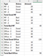
I want to have a formula that I can drag down rows (in Column C) that will return the sum of a group of another column (Column B) based on a blank cell between the groups (Column B). The groups vary in size (my example shows 3 and 4 categories), with some having 2 to 7 categories within a grouping. I have oversimplified then table for the Forum Members use. I will change the formula as necessary to differing columns or changes in formula operations (e.g. sum to percentage calculations), but I need to BASE formula to start with. I have tried numerous ways and failed. Also, looking for the formula to be in a single cell and not rely on a 'helper column'.

For the cells in Column C between totals, I want it to return blank (or ""), as I want to be able to drop the formula into any spreadsheet provided to me and put the formula at the top and drag to obtain quick results to report on.

I hope this is not too much a lift and the members can help. Thank you again. See sample table below.

 

[Fluff]

I am using Office 365.

I suggest that you update your Account details (or click your user name at the top right of the forum) so helpers always know what Excel version(s) & platform(s) you are using as the best solution often varies by version. (Don’t forget to scroll down & ‘Save’)

How about

=IF(B2="",SUM(C$2:C2)-SUM(D$1:D1),"")

 

[hagia_sofia]

Another option:

=LET(
r,C2:C19,
a,SCAN(0,r,LAMBDA(x,y,IF(y="",0,x+y))),
b,VSTACK(0,DROP(a,-1)),
IF(r<>"","",b))

 

[JamesCanale]

pile on:

MrExcelPlayground23.xlsx
	A	B	C	D
1	Type	Status	amount
2	a	x	20
3	b	x	40
4	c	x	30
5	total 1			90
6	a	t	20
7	b	t	10
8	c	t	10
9	total 2			40
10	q	x	50
11	w	x	10
12	e	x	30
13	r	x	40
14	total 3			130
15	q	t	10
16	w	t	10
17	e	t	20
18	r	t	50
19	total 4			90
Sheet28

Cell Formulas
Range	Formula
D2	D2	=IF(C2<>"","",SUM(DROP(C1:C$2,IFNA(XMATCH(,C1:C$2,0,-1),0))))
D3:D19	D3	=IF(C3<>"","",SUM(DROP(C$2:C2,IFNA(XMATCH(,C$2:C2,0,-1),0))))

Someday AI will be better at this. But today is not that day.

 

[secrestj]

Wow - as usual, the Forum Member pull through. I thank Fluff for the recommendation on updating my account and formula; I am running with JamesCanale's version, as I understand it - thank you. However, I just ran hagia_sofia version and amazing - I am going to do much more research in breaking down this formula and its potential future applications - I am always learning from everyones' various approaches to the same problem.

Thank you for each of your efforts. This is a great forum.

 

[Fluff]

Glad we could help & thanks for the feedback.

I am running with JamesCanale's version, as I understand it

Does that mean you don't understand the formula I suggested?

 

[secrestj]

Glad we could help & thanks for the feedback.


Does that mean you don't understand the formula I suggested?

No - you misunderstood. I went with the JamesCanale version, as I believe I can adapt it for my other formula changes I need. I am still working it to see if it works for me. Thank you for your follow up.

 

[secrestj]

Well, that was me being 'twice as smart by half'. While I was able to adapt the formula, I learned that by providing an over simplified example, the three working formulas did not work when adapted to my specific use.

A	B	C	D	E
1	Type	Status	Amount	%	Valid/Fail
2	MF - 1	Good	20	95.0%
3	MF - 2	Good	40	88.0%
4	MF - 3	Good	30	92.0%
5	Total Good MF	90	90.9%	VALID
6	MF - 1	Bad	20	82.0%
7	MF - 2	Bad	10	84.0%
8	MF - 3	Bad	10	73.0%
9	Total Bad MF	40	80.3%	VALID
10	Office - 1	Good	50	94.0%
11	Office - 2	Good	10	94.0%
12	Office - 3	Good	30	91.0%
13	Office - 4	Good	40	92.0%
14	Total Good Office	130	92.7%	VALID
15	Office - 1	Bad	10	71.0%
16	Office - 2	Bad	10	83.0%
17	Office - 3	Bad	20	78.0%
18	Office - 4	Bad	50	77.0%
19	Total Bad Office	90	77.2%	VALID

E5	=IF(ABS(SUMPRODUCT(C2:C4,D2:D4)/C5-D5)>0.01,"FAIL","VALID")
E9	=IF(ABS(SUMPRODUCT(C6:C8,D6:D8)/C9-D9)>0.01,"FAIL","VALID")
E14	=IF(ABS(SUMPRODUCT(C10:C13,D10:D13)/C14-D14)>0.01,"FAIL","VALID")
E19	=IF(ABS(SUMPRODUCT(C15:C18,D15:D18)/C19-D19)>0.01,"FAIL","VALID")

I am attempting to 'validate' the weighted average is within a specific tolerance of error. The thought is to have the formula to be placed in the Column E and drag to the bottom of the rows, as the quantity of rows varies, but the blank cells in Column B are consistent. I was not able to adapt the prior formula suggestions to my need and am return with hat in hand requesting more assistance. Answers are only as good as the questions; so, this version is to improve my question. Thank you again in advance.

 

[secrestj]

I just realized that my table did not copy correctly from excel as my example. I have retyped the table in the correct format that I am analyzing the data. The table represents real estate type and their statuses, followed by quantity and occupancy. The 'Total' rows (5,9,14,19 - in the sample below) represent the weighted average in the percentage column.

I want to create a formula in column E that allows me to copy/paste new data in columns A, B, C, D and columns E will adjust to the new quantity of the data sets (with the format and columns A, B, C, D being the same). For example, sometimes the quantity of multi-family data set has 2, 4, 5 rows rather than 3 rows in this example below. The goes with 'office' and sometimes there is 'retail (or other real estate types).
As such, I am trying for a formula that is already in Column E (adjusting to the change in Column A-D data) and I can drag the formula down if there are more rows in the data set. Also, I am validating the weighted average formula is calculating correctly and not relying on the data totals in columns C and D.

My current formula (before considering this change) is the following, but it is not dynamic to grow/contract with the quantity (row) changes of MF, Office, etc. and I go into the formula and add/reduce rows in the formulas on each of the total rows in column E.

E6	=IF(ABS(SUMPRODUCT(C3:C5,D3:D5)/C6-D6)>0.01,"FAIL","VALID")

Then, I started with a formula that only displays calculations in Column E based on an if statement, but cannot figure out the how to make a formula that runs the calculation based on the rows between the two 'blank' cells of column B, which is the only consistent pattern I can think of to base the dynamic calculations and make it drag-able down column E if there is more data provided.

E6	=IF(OR(AND(ISTEXT($A6),$B6=""),AND($A6="",$B6="")),"", ???????????????????

	A​	B​	C​	D​	E​
1​	Type	Status	Amount	%	Valid/Fail
2	Commercial RE
3​	MF-1	Good	20	95.0%
4​	MF-2	Good	40	88.0%
5​	MF-3	Good	30	92.0%
6​	Total Good MF		90	90.9%	VALID
7​	MF-1	Bad	20	82.0%
8​	MF-2	Bad	10	84.0%
9​	MF-3	Bad	10	73.0%
10​	Total Bad MF		40	80.3%	VALID
11​	Office-1	Good	50	94.0%
12​	Office-2	Good	10	94.0%
13​	Office-3	Good	30	91.0%
14​	Office-4	Good	40	92.0%
15​	Total Good Office		130	92.7%	VALID
16​	Office-1	Bad	10	71.0%
17​	Office-2	Bad	10	83.0%
18	Office-3	Bad	20	78.0%
19	Office-4	Bad	50	77.0%
20	Total Bad Office		90	77.2%	VALID

If you can help figure this formula out, I would greatly appreciate it. Thank you.

 

[Fluff]

As this is a totally different question, it needs a new thread. Thanks