Formula that pulls from a specific row for each month & "locks" into that row for the month?

[SirGruffles]

Apologies if this looks/sounds messy...

In the middle of my (probably unnecessarily complex/large) formula, I have this function: (OFFSET(INDIRECT(ADDRESS(ROW(), COLUMN())),-ROW()+2,0))
As it stands, this will pull the value of the cell 2 rows from the top, in the same column as the current cell.
While this works great for the first "area" of data (January 2020 in this instance), if I copy it down into the sections for other months, it will continue to pull January data only.

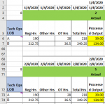
I attached a fragment of the worksheet to this post for some visual assistance.

The type of formula I'm looking for, in words I can only hope I'm using correctly:
1) Would function similarly to what's currently there, but
2) Would allow for pasting down into other months
a) In the picture, the 39 & 134 are correct in the January area, but are incorrect for the February area, as February has not occurred yet. It is still pulling that 1/4/2020 date value from the 2nd row.
b) Using a different variation of OFFSET... allowed me to easily code the "future" months, but gave me issues when pasting down the line of the current month. As going from Row 6 to Row 7 would take the OFFSET cell's value a cell down.

Is there a different way to use OFFSET and ADDRESS that would allow me to "lock" that specific month row (rows 2 & 69 in the picture) in their respective months? (Instead of my -ROW()+2 formula).

If more of the formula is needed for clarity, let me know and I can post more.

The goal here is to create a formula I can use in each month's sections, and not having to create a different one for each month OR for each line (A,B,etc).

I appreciate any advice, tips, ideas.

Thank you for your time.

 

[CSmith]

An EXACT number offset sounds like what you want but without more data and better explanation not much more I can offer

 

[SirGruffles]

What other data would you like to see?

If by "exact" number offset, you mean something to the effect of: OFFSET(cell,-4,0)?

In the attached image from the post, the same formula are in the yellow cells.
But because of the (OFFSET(INDIRECT(ADDRESS(ROW(), COLUMN())),-ROW()+2,0)), it's always hitting that "1/4/2020" in cell F2.
Even when I paste the formula into the February section, it will still pull the value of cell F2.

Is there a way to get this offset formula (or a variation of it) that would allow me to paste into the cell in F73, so that it would pull the data from F69?
But going past that, so that when I drag it down to F74, it will still pull the data from F69?

 

[Peter_SSs]

Can you give us the whole formulas that are in F6 & F7?

What version of Excel are you using?

 

[SirGruffles]

Oh boy...I sure can....please don't judge me too hard:

F6: =IFERROR(IF(MONTH((OFFSET(INDIRECT(ADDRESS(ROW(), COLUMN())),-ROW()+2,0))-7)=MONTH((OFFSET(INDIRECT(ADDRESS(ROW(), COLUMN())),-ROW()+2,-22))),SUMIFS(INDEX('Daily Dashboard Datalink V2'!$E:$KZ,MATCH($B6&P$5,'Daily Dashboard Datalink V2'!$A:$A,0),0),'Daily Dashboard Datalink V2'!$E$2:$KZ$2,"<="&(OFFSET(INDIRECT(ADDRESS(ROW(), COLUMN())),-ROW()+2,0)),'Daily Dashboard Datalink V2'!$E$2:$KZ$2,">"&(OFFSET(INDIRECT(ADDRESS(ROW(), COLUMN())),-ROW()+2,0))-6)),SUMIFS(INDEX('Daily Dashboard Datalink V2'!$E:$KZ,MATCH($B6&P$5,'Daily Dashboard Datalink V2'!$A:$A,0),0),'Daily Dashboard Datalink V2'!$E$2:$KZ$2,"<="&((OFFSET(INDIRECT(ADDRESS(ROW(), COLUMN())),-ROW()+2,0))),'Daily Dashboard Datalink V2'!$E$2:$KZ$2,">"&((OFFSET(INDIRECT(ADDRESS(ROW(), COLUMN())),-ROW()+2,0))-DAY(OFFSET(INDIRECT(ADDRESS(ROW(), COLUMN())),-ROW()+2,0))+1)))

F7: =IFERROR(IF(MONTH((OFFSET(INDIRECT(ADDRESS(ROW(), COLUMN())),-ROW()+2,0))-7)=MONTH((OFFSET(INDIRECT(ADDRESS(ROW(), COLUMN())),-ROW()+2,-22))),SUMIFS(INDEX('Daily Dashboard Datalink V2'!$E:$KZ,MATCH($B7&P$5,'Daily Dashboard Datalink V2'!$A:$A,0),0),'Daily Dashboard Datalink V2'!$E$2:$KZ$2,"<="&(OFFSET(INDIRECT(ADDRESS(ROW(), COLUMN())),-ROW()+2,0)),'Daily Dashboard Datalink V2'!$E$2:$KZ$2,">"&(OFFSET(INDIRECT(ADDRESS(ROW(), COLUMN())),-ROW()+2,0))-6)),SUMIFS(INDEX('Daily Dashboard Datalink V2'!$E:$KZ,MATCH($B7&P$5,'Daily Dashboard Datalink V2'!$A:$A,0),0),'Daily Dashboard Datalink V2'!$E$2:$KZ$2,"<="&((OFFSET(INDIRECT(ADDRESS(ROW(), COLUMN())),-ROW()+2,0))),'Daily Dashboard Datalink V2'!$E$2:$KZ$2,">"&((OFFSET(INDIRECT(ADDRESS(ROW(), COLUMN())),-ROW()+2,0))-DAY(OFFSET(INDIRECT(ADDRESS(ROW(), COLUMN())),-ROW()+2,0))+1)))

As for version, I'm seeing Excel for Office 365 MSO - 64 bit.
I'm not seeing a year version...my apologies.

 

[SirGruffles]

In my desire to reply as quick as possible, I neglected to remember that F6/F7 are indeed the same formula.

 

[Peter_SSs]

please don't judge me too hard

OK, yes, they are rather cumbersome.

I had hoped to offer a whole alternative formula but I am not able to replicate what you have or want as I also don't have the 'Daily Dashboard Datalink V2' sheet & its data.
Never-the-less, see if this is some help. If all your sections have the word "Actual" 2 rows below the row you want to access with your formula (or we could use 'Processed Output' 3 rows below) then you can use a formula like I have shown in F6, drag/copy it to F7 then copy both and paste in F73:F74 and any other sections to pick up that sections date.

Book1
	F
1
2	1/04/2020
3	2
4	Actual
5	Processed Output
6	1/04/2020
7	1/04/2020
66
67
68
69	2/08/2020
70	5
71	Actual
72	Processed Output
73	2/08/2020
74	2/08/2020
75
Sheet1

Cell Formulas
Range	Formula
F6:F7	F6	=INDEX(F$1:F5,AGGREGATE(14,6,(ROW(F$1:F5)-ROW(F$1)+1)/(F$1:F5="Actual"),1)-2)

 

[SirGruffles]

Let me give this a try and come back (hopefully) shortly.

I'm afraid of posting the entire file, both due to overall size, but also feel like it's a breach of "security" of my company to divulge so much production info.
I can try to shrink and rename as much as possible if your above solution doesn't pan out.

Thank you for your time.

 

[Peter_SSs]

Shouldn't need the whole file. If you can't adapt what I have given you, perhaps you could make a very small file with dummy data to replicate what is required. If we get to that, please don't just post images as we cannot copy from those to test. XL2BB (see my signature block below) is one way to post small sample data (that we can copy) directly here in the forum.

 

[SirGruffles]

Sweet baby Jesus....it works! It's perfect! ?
This **** spreadsheet is finally as dynamic as I can make it, with the formatting being "locked" by upper management.

Now, I need to go read up on this Aggregate function, as I've never used this one before...

(and noted on the XL2BB for sample data tables. will do so in the future)

Thank you so much for your help on this.
This has been driving me crazy for the past week and a half.

Do I need to do anything to mark as "solved"?