Formula returning #VALUE! help

[cmajor335]

Hello all, apologies for the long post but it was difficult to describe.
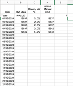
I have three columns, "B", "C" and "N". Both B & N columns contain mileage, "B3" is the start mileage and "N" the end mileage in each cell "3" to "33" for a day of the month.
Cell value "B3" = 19837.
Each Cell in COL "N" has the end mileage for the date, but until the month ends the following days replicate the last date's end mileage. E.G. if "N7" = 19842, all following cells "N8:N33" will also show 19842.
Column "C" is a column where data is entered manually, as using Column "B" doesn't work as it contains a formula.
In B2 the current formula = N33 - B3 will give me the total daily mileage.
"B3" equals 1st of the month and row 7 equals 4th of the month, going down to row 33. I can replicate the following cells in Row "N" with the last data from Row "N7" but thinks it spoils the spreadsheet.
To find the last "N" row with data I have another cell S2 with the formula =MATCH(TRUE,ISBLANK(C3:C34),0)+1. I couldn't combine this in a formula for "B2".
My Formula in cell "B2" is =("N"&S2)-B3 this returns #VALUE! yet when I highlight "N"&S2 in cell "B2" it returns me "N7".
The formula N7-B3 returns '5'which is the answer I should have in "B2".

 

[Sufiyan97]

Hi & Welcome to MrExcel.

Can you post the data along with some manually typed expected results.

MrExcel has a tool called “XL2BB” that lets you post samples of your data that will allow us to copy/paste it to our Excel spreadsheets, so we can work with the same copy of data that you are. Instructions on using this tool can be found here: XL2BB Add-in

Note that there is also a "Test Here” forum on this board. This is a place where you can test using this tool (or any other posting techniques that you want to test) before trying to use those tools in your actual posts.

Also give this a try in B2

=INDIRECT("N"&S2)-B3

 

[Fluff]

How about

=index(n:n,s2)-b3

 

[cmajor335]

Hi & Welcome to MrExcel.

Can you post the data along with some manually typed expected results.

MrExcel has a tool called “XL2BB” that lets you post samples of your data that will allow us to copy/paste it to our Excel spreadsheets, so we can work with the same copy of data that you are. Instructions on using this tool can be found here: XL2BB Add-in

Note that there is also a "Test Here” forum on this board. This is a place where you can test using this tool (or any other posting techniques that you want to test) before trying to use those tools in your actual posts.

Also give this a try in B2

=INDIRECT("N"&S2)-B3

Both replies have worked, thank you so much. I have now managed (Age and lack of using EXCEL like this for many years don't help ) to download the Xl2bb add-on so will be better equipped

 

[cmajor335]

How about

=index(n:n,s2)-b3

Both replies have helped, many thanks.

 

[cmajor335]

Thank you all, as usual, the experts are very quick to help. Please do not post any more answers as the ones above have done the job.
Best Wishes
Graham

 

[Fluff]

Glad we could help & thanks for the feedback.

 

[cmajor335]

Glad we could help & thanks for the feedback.

I like to thank people for any help given, whether on line or in person. It is good that there is a site/forum like this where people do not judge other people's lack of experience.

 

[Peter_SSs]

Please do not post any more answers as the ones above have done the job.

That's fine that you are happy with what has been provided but future readers looking for something similar may be interested if other solutions come along so we don't stop people from continuing to make suggestions.

For example, if I have understood correctly, unless the S2 formula is needed for something else as well, it could be removed (tidier worksheet) and B2 could have this:

=LOOKUP(9^9,N:N)-B3

 

[Sufiyan97]

Hi @Peter_SSs

I tried your formula by putting text and numbers, it takes last filled number in column N and that's interesting.

Can we use for text as well? and for both numbers and text? if so how to do that?