Formula between Sheets

[mirofa]

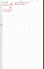
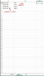
Greetings. I'm new here and I don't have much time to read each post one by one. I will give you an example in text and I will leave photos under text.
I have two sheets. In the SHEET 2 I have columns A and B. In column A I have numbers (codes) and in the second column B names of those codes.
I want in SHEET 1 , column A , in any cell for example In the first 15 when I enter numbers (codes) from SHEET 2 that it automatically recognizes name of that number (codes) from SHEET 2.
So that I don't have to manually type the name every time after i write number ( codes) . Note: Each number (code) is different and each of them has a different name.
Is that possible and thanks in advance.

 

[Trebor76]

Hi mirofa,

Welcome to MrExcel!!

Put this formula into cell B1 of SHEET 1 and copy down as far as need:

=IFERROR(VLOOKUP(A1,'SHEET 2'!A:B,2,FALSE),"")

Hope that helps,

Robert

 

[mirofa]

=IFERROR(VLOOKUP(A1,'SHEET 2'!A:B,2,FALSE),"")

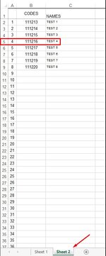
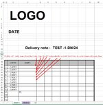
It shows me this error. I'm trying to create a packing slip. I'll try to explain better. In Sheet 2 I have product codes and names. And when I enter the product code in sheet 1 for example in cell B2 or B3 , I want it to immediately write the name of the product that is related to that code in the column next to it, so that I don't have to manually enter names every time. Look at new pictures.

thank you

 

[RoryA]

It may be a regional settings issue - perhaps you normally use semicolons rather than commas as argument separators? Try:

=IFERROR(VLOOKUP(A1;'SHEET 2'!A:B;2;FALSE);"")

 

[mirofa]

It may be a regional settings issue - perhaps you normally use semicolons rather than commas as argument separators? Try:

=IFERROR(VLOOKUP(A1;'SHEET 2'!A:B;2;FALSE);"")

I solved it. Thank you very much.