Formatting pivot tables

[Walkon]

Good afternoon,

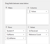
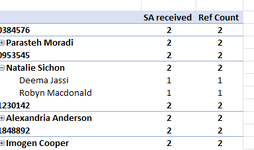
A colleague formatted a pivot table for me last year and when I have tried to re-create the formatting it looks very different. Please see images. The image titled Preferred Format 1 is how it looked when he did it. In that example, each of the following items is in its own column: Student #, Full Name, RFullName (reference full name), SA received, and Ref Count. Further, RFullName(s) only appears when the +/- button next to the Fullname is set to -. His field settings can be seen in the image titled Preferred Format 2.
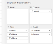
When I tried to replicate the format, I included the field names in the same areas as he had done (see image titled UN-preferred format 2) however, in my pivot table, rather than having the student number, the Full, Name and the RFullName in separate columns, they are all in the same column (see image titled UN-Preferred format 1).
Any suggestions as to how to replicate his formatting greatly appreciated.

 

[johnny51981]

My best guess would be that they used Classic Mode.

In order to do that, right click on the PivotTable, select PivotTable Options. Select the View Tab. Check the box next to "Classic PivotTable layout...". And then click OK.

 

[Walkon]

My best guess would be that they used Classic Mode.

In order to do that, right click on the PivotTable, select PivotTable Options. Select the View Tab. Check the box next to "Classic PivotTable layout...". And then click OK.
View attachment 95150

My best guess would be that they used Classic Mode.

In order to do that, right click on the PivotTable, select PivotTable Options. Select the View Tab. Check the box next to "Classic PivotTable layout...". And then click OK.
View attachment 95150

Thank-you very much! That worked perfectly. Greatly appreciated.

 

[johnny51981]

YAY!

 

[Walkon]

Good afternoon,

A colleague formatted a pivot table for me last year and when I have tried to re-create the formatting it looks very different. Please see images. The image titled Preferred Format 1 is how it looked when he did it. In that example, each of the following items is in its own column: Student #, Full Name, RFullName (reference full name), SA received, and Ref Count. Further, RFullName(s) only appears when the +/- button next to the Fullname is set to -. His field settings can be seen in the image titled Preferred Format 2.
When I tried to replicate the format, I included the field names in the same areas as he had done (see image titled UN-preferred format 2) however, in my pivot table, rather than having the student number, the Full, Name and the RFullName in separate columns, they are all in the same column (see image titled UN-Preferred format 1).
Any suggestions as to how to replicate his formatting greatly appreciated.

YAY!

Perhaps I can bother you for with one more quick question?
Now when I click the +/- button the RFullName(s) appear in their own column (thanks!) but the first one displays one row down from the FullName (see image titled UN-preferred 3). In the Preferred format the first one appeared on the same line (see image titled Preferred 1), which is a significant space saver. I've tried a few of the options that appear when I right click as you showed me earlier, but with no luck so far. Any suggestions as to how to make this happen greatly appreciated.

 

[johnny51981]

That would indicate that, in your PivotTable's Source Data, Natalie has a blank RFullName. Where they had no blanks in Preferred Format.

 

[Walkon]

That would indicate that, in your PivotTable's Source Data, Natalie has a blank RFullName. Where they had no blanks in Preferred Format.

Hi again,

I do appreciate the quick replies, and am sorry to bother you. I have a ttached a copy of the data table that I beleive the data is being pulled from. See image RFullName data table.

 

[johnny51981]

Ok. Filter for Natalie in the AFulName. Then look to see if there are any empty/null cells in the RFullName column.

Any empties would be the reason why that extra row is being added to the pivot table

 

[Walkon]

Ok. Filter for Natalie in the AFulName. Then look to see if there are any empty/null cells in the RFullName column.

Ok. Filter for Natalie in the AFulName. Then look to see if there are any empty/null cells in the RFullName column.

Any empties would be the reason why that extra row is being added to the pivot table

Any empties would be the reason why that extra row is being added to the pivot table

I think I have filtered as suggested - see image. I filtered the data table.

 

[Walkon]

I think I have filtered as suggested - please see attached image. I filtered the data table. I don't see any blanks. Is this where you wanted me to filter?