Find used items between out and returned

[bobbieatendido]

Hello,

Is there a way to find "used" products from my list of "out" products and "returned" products?

Notes:

• "out" and "returned" products may have the same product code
• we ship "out" about 100 products (some have the same product codes) and they "return" 90 products

Example:

OUT	RETURNED	USED
Product a1	Product a1	Product a1
Product a1	Product b2	Product c3
Product b2	Product d4
Product c3	Product e5
Product d4	Product c3
Product e5
Product c3

What I "out" from my inventory was:
2pcs Product a1
1pc Product b2
2pcs Product c3
1pc Product d4
1pc Product e5

Then they "returned" 1pc of each, so what was used was 1pc of Product a1 and c3. However in our case, we ship out 1, 2 or even 10 of the same product code and it could reach up to 50 products "out".

Thank you very much for your help.

 

[Eric W]

Try:

Book1
	A	B	C
1	OUT	RETURNED	USED
2	Product a1	Product a1	Product a1
3	Product a1	Product b2	Product c3
4	Product b2	Product d4
5	Product c3	Product e5
6	Product d4	Product c3
7	Product e5
8	Product c3
9
Sheet5

Cell Formulas
Range	Formula
C2:C8	C2	=IFERROR(INDEX($A:$A,AGGREGATE(15,6,ROW($A$2:$A$8)/((COUNTIF(OFFSET($A$2,0,0,ROW($A$2:$A$8)-ROW($A$2)+1),$A$2:$A$8))>COUNTIF($B$2:$B$8,$A$2:$A$8)+COUNTIF($C$1:$C1,$A$2:$A$8)),1)),"")

Please update your member profile with the version of Excel you're using. It's possible that there's a better answer if you have a newer version of Excel with some new functions.

 

[Eric W]

Here's a version that should work with Excel 365:

Book1
	A	B	C
1	OUT	RETURNED	USED
2	Product a1	Product a1	Product a1
3	Product a1	Product b2	Product c3
4	Product b2	Product d4
5	Product c3	Product e5
6	Product d4	Product c3
7	Product e5
8	Product c3
9
Sheet5

Cell Formulas
Range	Formula
C2:C3	C2	=FILTER(A2:A8,COUNTIF(OFFSET(A2,0,0,ROW(A2:A8)-ROW(A2)+1),A2:A8)>COUNTIF(B2:B8,A2:A8))
Dynamic array formulas.

 

[bobbieatendido]

Hi Eric,

Thank you; I have updated my info. I'm using Microsoft 365.

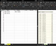
I'm not sure if its working because it is not showing the products. Also, it seems to slow down the program when I input a lot of products.

I input product codes on column F. (product codes are on the right side of the photo "database" sheet)
When the products return, I input all of them on column I
and whatever was not returned, it should show up on column L.

Thank you.

 

[Eric W]

Which formula are you using? Can you show a sample of your sheet using XL2BB, or at least another screen print like you did before? I'm wondering if the products are spelled exactly the same.

When you say, "a lot of products", how many is that? This is a reasonably computational-intensive formula, so on large ranges, it could slow down your sheet. You may be better served with a macro.

 

[bobbieatendido]

Input Sheet
Column F: no formula
Column G: =vlookup product name of column F
Column I: no formula
Column J: =vlookup product name of column I
Column L: no formula
Column M: =vlookup product name of column L
Column N: =IF(L2 <>"",1,) - Column N just shows 1 everytime we barcode something on Column L. (we barcode 2 products with the same product code and it will still count as 1)

Database Sheet
Column A: Control Number
Column B: Product Code
Column C: Product Name
Column D: Product Price

• I'm wondering if the products are spelled exactly the same.
  • Yes they are, but they are product codes (101-111, the vlookup (on column G, J and M) is to show what product it is)
• When you say, "a lot of products", how many is that?
  • We can ship up to 1000+ products in one single shipment order
• You may be better served with a macro.
  • I think so too, is there a way to do this automatically without clicking a button?

Thank you.

Column K: is just to double check if quantity of Column F (shipped out) - Column I (returned) = Column L (used products) is correct.
To eliminate this I wanted to automatically populate Column L (used) with Column F (shipped out) - Column I (returned)

xl2bb:

Sample.xlsx
	F	G	H	I	J	K	L	M	N
1		Shipped			Returned		Code	Product Used	QTY
2	110-123	S, H, PS, #0, Sz8		110-124	S, H, PS, #1, Sz9		110-123	S, H, PS, #0, Sz8	1
3	110-124	S, H, PS, #1, Sz9		110-125	S, H, PS, #2, Sz10		110-127	S, H, PS, #3, Sz10	1
4	110-125	S, H, PS, #2, Sz10		110-126	S, H, PS, #2, Sz11
5	110-126	S, H, PS, #2, Sz11
6	110-127	S, H, PS, #3, Sz10
Input

Cell Formulas
Range	Formula
K1:K6	K1	=$D$36-$D$37
J2:J6	J2	=IFERROR(VLOOKUP(I2,Database!B:D,2,FALSE),0)
M2:M6	M2	=IFERROR(VLOOKUP(L2,Database!B:D,2,FALSE),0)
N2:N6	N2	=IF(L2 <>"",1,)
G2:G6	G2	=IFERROR(VLOOKUP(F2,Database!B:D,2,FALSE),0)

Cells with Conditional Formatting
Cell	Condition		Cell Format	Stop If True
K1:K40,O1:O40	Cell Value	<>$D$38	text	NO

 

[bobbieatendido]

Example
We shipped:
2pcs Sz8
3pcs Sz9
1pc Sz10
1pc Sz11

They returned:
1pc Sz8
2pcs Sz9
1pc Sz10

on Column L, it should auto-populate:
1pc Sz8
1pc Sz9
1pc Sz11

Every cell is locked except Column F and Column I, so we cant accidentally ruin the formulas.
we only input the product codes on Col F (shipped) and Col I (returned)
Column L should just auto-populate what is missing in Column I from Column F

Thank you so much!

Sample.xlsx
	F	G	H	I	J	K	L	M	N
1		Shipped			Returned		Code	Product Used	QTY
2	110-123	S, H, PS, #0, Sz8		110-123	S, H, PS, #0, Sz8		110-123	S, H, PS, #0, Sz8	1
3	110-123	S, H, PS, #0, Sz8		110-124	S, H, PS, #1, Sz9		110-124	S, H, PS, #1, Sz9	1
4	110-124	S, H, PS, #1, Sz9		110-124	S, H, PS, #1, Sz9		110-126	S, H, PS, #2, Sz11	1
5	110-124	S, H, PS, #1, Sz9		110-125	S, H, PS, #2, Sz10
6	110-124	S, H, PS, #1, Sz9
7	110-125	S, H, PS, #2, Sz10
8	110-126	S, H, PS, #2, Sz11
Input

Cell Formulas
Range	Formula
K1:K8	K1	=$D$36-$D$37
J2:J8	J2	=IFERROR(VLOOKUP(I2,Database!B:D,2,FALSE),0)
M2:M8	M2	=IFERROR(VLOOKUP(L2,Database!B:D,2,FALSE),0)
N2:N8	N2	=IF(L2 <>"",1,)
G2:G8	G2	=IFERROR(VLOOKUP(F2,Database!B:D,2,FALSE),0)

Cells with Conditional Formatting
Cell	Condition		Cell Format	Stop If True
K1:K40,O1:O40	Cell Value	<>$D$38	text	NO

 

[Eric W]

After adjusting for the different locations, the formula seems to work fine:

Book1
	F	G	H	I	J	K	L	M	N
1		Shipped			Returned		Code	Product Used	QTY
2	110-123			110-123			110-123		1
3	110-123			110-124			110-124		1
4	110-124			110-124			110-126		1
5	110-124			110-125
6	110-124
7	110-125
8	110-126
9
Sheet7

Cell Formulas
Range	Formula
L2:L4	L2	=FILTER(F2:F1000,(F2:F1000<>"")*(COUNTIF(OFFSET(F2,0,0,ROW(F2:F1000)-ROW(F2)+1),F2:F1000)>COUNTIF(I2:I1000,F2:F1000)))
N2:N4	N2	=IF(L2#>0,1)
Dynamic array formulas.

I also tested with up to 1000 items in columns F and I, and the formula still computed almost instantaneously. Let me know how it works for you.

 

[bobbieatendido]

It absolutely works!
Thank you sooooo much!