Find more recurring text in same column but skip specific cells?

bmsmith311

New Member
Joined
May 1, 2022
Messages
12
Office Version
  1. 2019
Platform
  1. MacOS
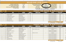
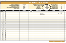
Hi there! I made a spreadsheet and I'm trying to have it autocalculate data, but I'm looking to find the most often recurring text values. This spreadsheet is broken down by month and I'm trying to have one box give a "running total" for the year as the user fills in the data, but obviously we aren't going to have any data for the later months until later in the year so without placeholders, it'll throw an error code. Here is what I currently have:

Excel Formula:
=INDEX(I14:I450,MODE(IF(I14:I450<>"",MATCH(I14:I450,I14:I450,0))))
where the I column is showing a particular genre of a book that a person read. For this formula, as I understand it, I can't skip cells or select only certain ranges within the same column, so while it will ignore zero or blank, it's also including each month's totals (which will be errors until those months are filled in) and I think that's what's causing the error for my "grand total" cell.

Is there a way to skip cells that show an error? I tried a few things after a google search but none of them seemed to work.
Thank you!
 

Attachments

  • Screen Shot 2022-05-01 at 7.19.46 AM.png
    Screen Shot 2022-05-01 at 7.19.46 AM.png
    190.3 KB · Views: 28
  • Screen Shot 2022-05-01 at 7.20.35 AM.png
    Screen Shot 2022-05-01 at 7.20.35 AM.png
    126.1 KB · Views: 25

Excel Facts

Round to nearest half hour?
Use =MROUND(A2,"0:30") to round to nearest half hour. Use =CEILING(A2,"0:30") to round to next half hour.
The images are difficult to see, but if I'm not mistaken, column B has numbers on every row you want to consider, so you could consider using that to filter out blank rows and any summary rows that appear after each month (because those have nothing in column B). And then to suppress the error before anything is filled in, you could wrap the entire formula with an IFERROR to return a blank:
Excel Formula:
=IFERROR(INDEX(I14:I450,MODE(IF(ISNUMBER(B14:B450),MATCH(I14:I450,I14:I450,0)))),"")
 
Upvote 0
The images are difficult to see, but if I'm not mistaken, column B has numbers on every row you want to consider, so you could consider using that to filter out blank rows and any summary rows that appear after each month (because those have nothing in column B). And then to suppress the error before anything is filled in, you could wrap the entire formula with an IFERROR to return a blank:
Excel Formula:
=IFERROR(INDEX(I14:I450,MODE(IF(ISNUMBER(B14:B450),MATCH(I14:I450,I14:I450,0)))),"")
Thank you for your reply! I'm sorry the images are hard to see -- I ended up having to size them way down in order to be accepted ?

That seems like a brilliant work around! I tried the formula and it's not showing an error but it's just showing a blank cell. I was hoping to allow it to get the most common value entered so far so people would be able to see it as the year progresses. Open to any other suggestions! Thank you!
 
Upvote 0
Could you post the formula that you are using and confirm that column B does contain numbers? The formula worked fine in a small example worksheet that I made. For example, go to an empty cell and reference a "number" in column B and enter:
=TYPE(B29)
...and confirm that it returns a 1 (which means B29 is a number).
Absolutely! Here is a screenshot & the code I was using //
Excel Formula:
=IFERROR(INDEX(I14:I450,MODE(IF(ISNUMBER(B14:B450),MATCH(I14:I450,I14:I450,0)))),"")

And yes, confirmed that column B is registering as a number (performed the test and it did come back as 1).
Thank you!
 

Attachments

  • Screen Shot 2022-05-02 at 9.54.22 AM.png
    Screen Shot 2022-05-02 at 9.54.22 AM.png
    176 KB · Views: 18
Upvote 0
Does the range I14:I450 contain the Genres that you want to consider? If the range contains no data, the MODE/MATCH part of the formula would produce an error, and the IFERROR wrapping then displays a blank rather than the error message. Try removing the IFERROR wrapping...the IFERROR( and the ,"") at the beginning and end of the formula and let me know what you see. Here's a small mockup showing what mine looks like:
MrExcel_20220430.xlsx
BGHI
6Top GenreRomance
7
8
9
10
11
12Title Bar
13GENRE
14MONTH
151Mystery/Suspense
162Romance
173Mystery/Suspense
18Mystery/Suspense
19Something
20
21Title Bar
22GENRE
23MONTH
241Mystery/Suspense
252Biography
263Romance
274Mystery/Suspense
285Mystery/Suspense
296Romance
307Romance
318Romance
329Romance
33Mystery/SuspenseMystery/Suspense
34SomethingSomething
Sheet5
Cell Formulas
RangeFormula
I6I6=IFERROR(INDEX(I14:I450,MODE(IF(ISNUMBER(B14:B450),MATCH(I14:I450,I14:I450,0)))),"")
 
Upvote 0
Did the original formula you posted work okay? One other thing occurs to me...since you are using Excel 2019, was the formula entered as an array formula...with Ctrl-Shift-Enter? To try that, with the cell containing the formula selected, go the formula bar and hit Ctrl-Shift-Enter. Curly brackets should appear around the formula (they are not manually typed in).
 
Upvote 0
Does the range I14:I450 contain the Genres that you want to consider? If the range contains no data, the MODE/MATCH part of the formula would produce an error, and the IFERROR wrapping then displays a blank rather than the error message. Try removing the IFERROR wrapping...the IFERROR( and the ,"") at the beginning and end of the formula and let me know what you see. Here's a small mockup showing what mine looks like:
MrExcel_20220430.xlsx
BGHI
6Top GenreRomance
7
8
9
10
11
12Title Bar
13GENRE
14MONTH
151Mystery/Suspense
162Romance
173Mystery/Suspense
18Mystery/Suspense
19Something
20
21Title Bar
22GENRE
23MONTH
241Mystery/Suspense
252Biography
263Romance
274Mystery/Suspense
285Mystery/Suspense
296Romance
307Romance
318Romance
329Romance
33Mystery/SuspenseMystery/Suspense
34SomethingSomething
Sheet5
Cell Formulas
RangeFormula
I6I6=IFERROR(INDEX(I14:I450,MODE(IF(ISNUMBER(B14:B450),MATCH(I14:I450,I14:I450,0)))),"")
You are correct! And your example is exactly what I'm trying to get it to show. I removed the IFERROR portions and went back to this:
Excel Formula:
=(INDEX(I14:I450,MODE(IF(ISNUMBER(B14:B450),MATCH(I14:I450,I14:I450,0)))))

But I'm still getting the error. And yep, I had done CTRL SHIFT ENTER each time, so that shouldn't be an issue.
Do you think my "summary" boxes would be causing an issue? I used the same formula/concept at the bottom of each sub-divided section (so, each month) to show the summary after each month was over, but that's in the same column and I don't know if that would muddy things up since there are 12 of those it would have to sort through as well.
 
Upvote 0
The summary boxes (those that are shaded yellow-orange and gray in my post) should not be causing any issues because they are ignored due to the ISNUMBER filtering part of the formula. For example, in the example I posted, the entire IF function part of the formula returns the array:
{FALSE;2;3;2;FALSE;FALSE;FALSE;FALSE;FALSE;FALSE;2;12;3;2;2;3;3;3;3;FALSE;FALSE;FALSE;....followed by a lot more FALSE's out to array element 450-14+1}
This array represents the array element number where the first match is found for each item in the array. The FALSE elements represent the positions that are ignored. This array is passed to the MODE function where these array element numbers are evaluated and the most common one is returned...and this value is passed along to the INDEX function to return the value at that location in the array.

Try this version, which looks for "Yes" or "No" entries in column F. Only those rows will be considered.
Excel Formula:
=IFERROR(INDEX(I14:I450,MODE(IF(((F14:F450="Yes")+(F14:F450="No"))>0,MATCH(I14:I450,I14:I450,0)))),"")
 
Upvote 0
Got it! I didn't think it should make a difference but figured I'd throw it out there anyway. I tried the yes/no option you provided and it resulted in a display of "0"
The summary boxes (those that are shaded yellow-orange and gray in my post) should not be causing any issues because they are ignored due to the ISNUMBER filtering part of the formula. For example, in the example I posted, the entire IF function part of the formula returns the array:
{FALSE;2;3;2;FALSE;FALSE;FALSE;FALSE;FALSE;FALSE;2;12;3;2;2;3;3;3;3;FALSE;FALSE;FALSE;....followed by a lot more FALSE's out to array element 450-14+1}
This array represents the array element number where the first match is found for each item in the array. The FALSE elements represent the positions that are ignored. This array is passed to the MODE function where these array element numbers are evaluated and the most common one is returned...and this value is passed along to the INDEX function to return the value at that location in the array.

Try this version, which looks for "Yes" or "No" entries in column F. Only those rows will be considered.
Excel Formula:
=IFERROR(INDEX(I14:I450,MODE(IF(((F14:F450="Yes")+(F14:F450="No"))>0,MATCH(I14:I450,I14:I450,0)))),"")
 
Upvote 0

Forum statistics

Threads
1,224,823
Messages
6,181,175
Members
453,021
Latest member
Justyna P

We've detected that you are using an adblocker.

We have a great community of people providing Excel help here, but the hosting costs are enormous. You can help keep this site running by allowing ads on MrExcel.com.
Allow Ads at MrExcel

Which adblocker are you using?

Disable AdBlock

Follow these easy steps to disable AdBlock

1)Click on the icon in the browser’s toolbar.
2)Click on the icon in the browser’s toolbar.
2)Click on the "Pause on this site" option.
Go back

Disable AdBlock Plus

Follow these easy steps to disable AdBlock Plus

1)Click on the icon in the browser’s toolbar.
2)Click on the toggle to disable it for "mrexcel.com".
Go back

Disable uBlock Origin

Follow these easy steps to disable uBlock Origin

1)Click on the icon in the browser’s toolbar.
2)Click on the "Power" button.
3)Click on the "Refresh" button.
Go back

Disable uBlock

Follow these easy steps to disable uBlock

1)Click on the icon in the browser’s toolbar.
2)Click on the "Power" button.
3)Click on the "Refresh" button.
Go back
Back
Top