Extracting Multiple Value by Using Unique Value

[93arpan]

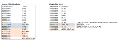
I'm working with a dataset that has two columns: Transaction (Column A) and Client ID (Column B). I'm aiming to extract the Client ID values associated with a specific Transaction from Column A.

For example, if I select Transaction 100000223, I want to retrieve the corresponding Client ID values, which are "IN AG, AT AG, and NL AG". Similarly, for Transaction 100000254, I'd like to obtain "PL AG and IN AG".

Column A (Transaction)	Column B (Client ID)
100000138	PL AG
100000145	OG AG
100000151	US AG
100000220	YU AG
100000223	IN AG
100000223	AT AG
100000223	NL AG
100000254	PL AG
100000254	IN AG

 

[alansidman]

Create a Parameter Query in Power Query

let
    Source = Excel.CurrentWorkbook(){[Name="Table1"]}[Content],
    #"Filtered Rows" = Table.SelectRows(Source, each ([Transaction] = Table2))
in
    #"Filtered Rows"

PQ Parameter.xlsx
	A	B	C	D	E	F	G	H	I	J
1	Transaction	Client ID		Transaction		Transaction	Client ID			Transaction
2	100000138	PL AG		100000145		100000145	OG AG			100000138
3	100000145	OG AG								100000145
4	100000151	US AG								100000151
5	100000220	YU AG		D1 is a lookup data validation from column J						100000220
6	100000223	IN AG		Once this has been entered, click on Data-->Refresh All						100000223
7	100000223	AT AG		Results are in columns F:G						100000254
8	100000223	NL AG
9	100000254	PL AG
10	100000254	IN AG
Sheet1

Cells with Data Validation
Cell	Allow	Criteria
D2	List	=$J$2:$J$7

 

[93arpan]

Create a Parameter Query in Power Query

let
    Source = Excel.CurrentWorkbook(){[Name="Table1"]}[Content],
    #"Filtered Rows" = Table.SelectRows(Source, each ([Transaction] = Table2))
in
    #"Filtered Rows"

PQ Parameter.xlsx
	A	B	C	D	E	F	G	H	I	J
1	Transaction	Client ID		Transaction		Transaction	Client ID			Transaction
2	100000138	PL AG		100000145		100000145	OG AG			100000138
3	100000145	OG AG								100000145
4	100000151	US AG								100000151
5	100000220	YU AG		D1 is a lookup data validation from column J						100000220
6	100000223	IN AG		Once this has been entered, click on Data-->Refresh All						100000223
7	100000223	AT AG		Results are in columns F:G						100000254
8	100000223	NL AG
9	100000254	PL AG
10	100000254	IN AG
Sheet1

Cells with Data Validation
Cell	Allow	Criteria
D2	List	=$J$2:$J$7

Thank you very much, I will try this using Power Query as majority of my transformation happens there, definitely going to try there
Also, outside Power query I found this excel formula helpful that gets the job done.
TEXTJOIN(", ",TRUE,UNIQUE(IF($A6=$A:$A,B:B,"")))

 

[myall_blues]

You could also use TEXTJOIN with FILTER

Book1
	A	B	C	D	E	F
1	Column A (Transaction)	Column B (Client ID)
2	100000138	PL AG		100000223	IN AG, AT AG, NL AG
3	100000145	OG AG		100000254	PL AG, IN AG
4	100000151	US AG
5	100000220	YU AG
6	100000223	IN AG
7	100000223	AT AG
8	100000223	NL AG
9	100000254	PL AG
10	100000254	IN AG
Sheet1

Cell Formulas
Range	Formula
E2:E3	E2	=TEXTJOIN(", ",TRUE,FILTER(B$2:B$10,A$2:A$10=D2))

 

[djclements]

With Excel for Microsoft 365, you could also try the new GROUPBY function. Some examples include:

=GROUPBY(A1:A10,B1:B10,ARRAYTOTEXT,3,0)

=GROUPBY(A1:A10,B1:B10,ARRAYTOTEXT,3,0,,A1:A10=100000223)

=GROUPBY(A1:A10,B1:B10,ARRAYTOTEXT,3,0,,(A1:A10>100000220)*(A1:A10<100000260))

=GROUPBY(A1:A10,B1:B10,ARRAYTOTEXT,3,0,,ISNUMBER(XMATCH(A1:A10,{100000223,100000254})))

Adjust the range references as needed; or, use an Excel table with structured references. For example:

=GROUPBY(Table1[[#All],[Transaction ID]],Table1[[#All],[Client ID]],ARRAYTOTEXT,3,0)