excel transpose text

[kfhw720]

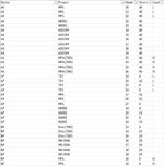
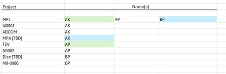
Hi, I have a spreadsheet which has 5 columns. I want it transposed by project, listing all the names of people working on that project in columns. On top of that I want anyone with an 'L' in column E to be highlighted in green (but only for the associated project) and same for anyone with an 'O' highlighted in blue. Can anyone help?

 

[hagia_sofia]

Hello, please test this:

a) transposed table:

=LET(
projects,B2:B36,
names,A2:A36,
u,UNIQUE(projects),
n,IFNA(DROP(REDUCE("",u,LAMBDA(a,b,VSTACK(a,TRANSPOSE(UNIQUE(FILTER(names,projects=b)))))),1),""),
HSTACK(u,n))

b) conditional formatting (adjust the first part of XLOOKUP based on your transposed table):

=XLOOKUP($F2&G2,$B$2:$B$36&$A$2:$A$36,$E$2:$E$36,"")="O"

=XLOOKUP($F2&G2,$B$2:$B$36&$A$2:$A$36,$E$2:$E$36,"")="L"

 

[kfhw720]

Thank you!
The first part works well, but for the formatting, which cell do I put the formula into? I don't really get that bit.

 

[hagia_sofia]

Thank you!
The first part works well, but for the formatting, which cell do I put the formula into? I don't really get that bit.

Highlight all the names in the new table and then go to conditional formatting and insert the formula (just adjust the first part of the formula, i.e. $F2&G2 base on the actual range of your transposed table where $F2 is the first project and G2 is the first name belonging to the first project).

 

[kfhw720]

amazing, thank you!

 

[kfhw720]

Sorry, one more thing. Do you know if there is anyway to keep formatting in the transpose? I.E. If I highlighted the names first before transposing the table.
And also if there is a way to ignore certain values of PROJECT? e.g. If PROJECT contains '[TBD]' then do not include in table.

 

[hagia_sofia]

As far as formatting is concerned, you can always copy and paste the format you need; as for the latter question, it is of course possible but what are the values you would like to exclude and how would you like to do it (to have a list of projects, drop-down menu...)?

 

[kfhw720]

I want it to list all projects in the result table, excluding any project which contains the text 'TBD'. Thank you!

 

[hagia_sofia]

Would this do the trick?

=LET(
projects,B2:B36,
names,A2:A36,
u,UNIQUE(FILTER(projects,ISNUMBER(FIND("TBD",projects))=FALSE)),
n,IFNA(DROP(REDUCE("",u,LAMBDA(a,b,VSTACK(a,TRANSPOSE(UNIQUE(FILTER(names,projects=b)))))),1),""),
HSTACK(u,n))

P. S. Please note that "FIND" is case sensitive, i.e. if it might happen that there will be some inconsistency (e.g. TbD), replace it with SEARCH.

 

[kfhw720]

AMAZING! thank you!