Dynamically pulling allowances and ignoring certain allowance for each employee

[hananak]

Dear All,

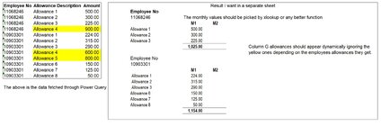
I have a file, in which the data tab fetches the data via Power Query in a table. There is second tab, in which we have to layout the data in a certain way to do some calculations for each employee based on the allowances they are getting. The complications are that certain allowances needs to be ignored when dynamically pulling the allowances and then use xlookup to pull the amounts from the data table based on allowances.

I have attached the picture, the first table reflects they way the data is there in the "Data tab" and the second table shows the way I want the result.

I hoping if this can be done either via Power query or Formulas, all I am trying to do is to avoid doing manual calculations.

Your help would be really appreciated.

Thanks.

 

[hagia_sofia]

Try:

=DROP(REDUCE("",F5:F7,LAMBDA(a,b,VSTACK(a,FILTER(C2:C13,(A2:A13=F3)*(B2:B13=b))))),1)

where F5:F7 you should replace with your actual list of allowances for particular employee, C2:C13 is amount, A2:A13 is the list of employee IDs, F3 is the ID of a particular employee and B2:B13 is the list of allowances.

 

[hananak]

Try:

=DROP(REDUCE("",F5:F7,LAMBDA(a,b,VSTACK(a,FILTER(C2:C13,(A2:A13=F3)*(B2:B13=b))))),1)

where F5:F7 you should replace with your actual list of allowances for particular employee, C2:C13 is amount, A2:A13 is the list of employee IDs, F3 is the ID of a particular employee and B2:B13 is the list of allowances.

Hi, Thanks for your reply.

I tried the formula but it's not working. I have attached the updated picture, which shows I want to have the list appear dynamically in column G for each employee based on their employee no. Suppose in G5, if I put employee no --> 10903301 then it should show all the allowances 1 to 8 except 4 & 5 and if I put employee no --> 11068246 in G5, it should show all the allowances, in this case Allowance 1 to 3, ignoring allowance 4.

I hope it's clear.

Thanks.

 

[hagia_sofia]

Oh, that is unfortunate. Just two questions: a) are you using the formula on 365? b) if the list of allowances shoud appear dynamically under employee name, what decides on which allowances should not be included?

 

[hananak]

Oh, that is unfortunate. Just two questions: a) are you using the formula on 365? b) if the list of allowances shoud appear dynamically under employee name, what decides on which allowances should not be included?

Yes am using Office 365 and currently it is fixed that allowance 4 and 5 will be excluded. But if we can make it dynamic based on a list, whatever allowances are on the list should be excluded, that would be amazing as in upcoming months, am seeing this change to be incorporated into the model.

Thanks.

 

[hagia_sofia]

I returned to the formula and tested it one more time and it is working just fine for me, returning an array of amounts. Apart from you testing it one more time (just to make sure that all ranges are where they should be) I do not know where the problem could be...

 

[hananak]

I returned to the formula and tested it one more time and it is working just fine for me, returning an array of amounts. Apart from you testing it one more time (just to make sure that all ranges are where they should be) I do not know where the problem could be...

In which cell I should put the formula G4?

 

[hananak]

I returned to the formula and tested it one more time and it is working just fine for me, returning an array of amounts. Apart from you testing it one more time (just to make sure that all ranges are where they should be) I do not know where the problem could be...

The formula is working but am not interested in getting the amounts, am interested in getting the allowances list dynamically ignoring allowance 4 and 5 for each employee.

 

[hagia_sofia]

My bad and therefore my apologies. Provided that you have a list of allowances that should be excluded for each employee, i.e. an Excel Table (to make it dynamic) with two columns, one being employee ID and the other the list of excluded allowances, try this (I tested it on employee 10903301):

=FILTER(FILTER(B2:B13,(A2:A13=G10)),BYROW(--(FILTER(B2:B13,(A2:A13=G10))=TRANSPOSE(FILTER(R2:R4,Q2:Q4=G10))),LAMBDA(a,SUM(a)))<>1)

where R2:R4 and Q2:Q4 is the list of allowances to be excluded (adjust according to your wishes).

 

[hananak]

My bad and therefore my apologies. Provided that you have a list of allowances that should be excluded for each employee, i.e. an Excel Table (to make it dynamic) with two columns, one being employee ID and the other the list of excluded allowances, try this (I tested it on employee 10903301):

=FILTER(FILTER(B2:B13,(A2:A13=G10)),BYROW(--(FILTER(B2:B13,(A2:A13=G10))=TRANSPOSE(FILTER(R2:R4,Q2:Q4=G10))),LAMBDA(a,SUM(a)))<>1)

where R2:R4 and Q2:Q4 is the list of allowances to be excluded (adjust according to your wishes).

The formula has an little issue, The R2:R4 and Q2:Q4 is the list of allowances to be excluded. For most of the employees, I have added the allowances to be excluded, then the formula works flawlessly but the moment there is an employee, who has no allowances that should be excluded and whatever the allowances they are getting is fine. The formula does not work because I did not put anything for this particular employee on the R2:R4 and Q2:Q4 - list of allowances, as there is nothing to exclude for them.

I would appreciate if you could fix it.

Thanks for your help!