mongoose00318
New Member
- Joined
- Feb 5, 2025
- Messages
- 4
- Office Version
- 365
- 2024
- 2021
- 2019
- Platform
- Windows
Hello, I am trying to create a way to quickly consolidate the data stored across 3 worksheets into one worksheet for analysis/charting purposes. I have uploaded images to try to help illustrate.
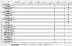
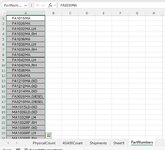
In worksheets PhysicalCount, AS400Count, & Shipments, the layout is the same as you can see in picture #1. Picture #3 is a named list called PartNumbers.
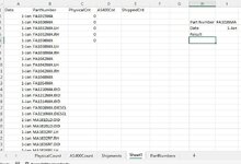
In image 2 I would like to do the following:
ColA = Incrementing dates for each part number (so after the data you see in picture 2, it would just repeat the same list of part numbers except move to Jan 2nd, etc). This will be used to reference the needed column in one of the first 3 worksheets
ColB = The part number used to reference the row in one of the 3 first worksheets
ColC = The result that is in worksheet "PhysicalCount" using the values in Sheet! columns A & B (ie. 1/1/25 & FA1015MA)
ColD = The result that is in worksheet "AS400Count" using the values in Sheet! columns A & B (ie. 1/1/25 & FA1015MA)
ColE = The result that is in worksheet "Shipments" using the values in Sheet! columns A & B (ie. 1/1/25 & FA1015MA)
I used =PartNumbers!$A$1:$A$32 in column B to dump the values in the named range "PartNumbers" and have got to here in column C: =PartNumbers!$A$1:$A$32
I have tried using match, xlookup, vlookup, etc and just can't figure out the combination but I know I am missing another vlookup or maybe it just needs to be an xlookup? I know Xlookup can only be used in 365 which is okay but if possible I would like something that is a little more cross compatible?
Any help would be greatly appreciated! Thank you all.
Sincerely,
J
In worksheets PhysicalCount, AS400Count, & Shipments, the layout is the same as you can see in picture #1. Picture #3 is a named list called PartNumbers.
In image 2 I would like to do the following:
ColA = Incrementing dates for each part number (so after the data you see in picture 2, it would just repeat the same list of part numbers except move to Jan 2nd, etc). This will be used to reference the needed column in one of the first 3 worksheets
ColB = The part number used to reference the row in one of the 3 first worksheets
ColC = The result that is in worksheet "PhysicalCount" using the values in Sheet! columns A & B (ie. 1/1/25 & FA1015MA)
ColD = The result that is in worksheet "AS400Count" using the values in Sheet! columns A & B (ie. 1/1/25 & FA1015MA)
ColE = The result that is in worksheet "Shipments" using the values in Sheet! columns A & B (ie. 1/1/25 & FA1015MA)
I used =PartNumbers!$A$1:$A$32 in column B to dump the values in the named range "PartNumbers" and have got to here in column C: =PartNumbers!$A$1:$A$32
I have tried using match, xlookup, vlookup, etc and just can't figure out the combination but I know I am missing another vlookup or maybe it just needs to be an xlookup? I know Xlookup can only be used in 365 which is okay but if possible I would like something that is a little more cross compatible?
Any help would be greatly appreciated! Thank you all.
Sincerely,
J