Dynamic MAXIFS

[jausfeld]

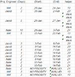
Effectively, any of the office 365 equations *IFS do not seem to dynamically update when new information is presented in the range, they stick to the first answer given and then just repeat. The real formula is quite long and it works well enough (though I'm sure there are faster ways). I have pasted it below for reference, but my question is about only a small part of this monstrosity.

=IF(U24=0,IF(BK24="","","NO PRIORITY"),IF(MINIFS(B:B,AG:AG,AG24)=U24,WORKDAY('2-Week'!$AH$31,0),IF(SMALL(B:B,2)=U24,WORKDAY(VLOOKUP(1,U:BM,45,FALSE),1,DropDowns!$F$2:$F$10),IF(SMALL(B:B,3)=U24,WORKDAY(VLOOKUP(2,U:BM,45,FALSE),1,DropDowns!$F$2:$F$10),IF(SMALL(B:B,4)=U24,WORKDAY(VLOOKUP(3,U:BM,45,FALSE),1,DropDowns!$F$2:$F$10),IF(SMALL(B:B,5)=U24,WORKDAY(VLOOKUP(4,U:BM,45,FALSE),1,DropDowns!$F$2:$F$10),IF(SMALL(B:B,6)=U24,WORKDAY(VLOOKUP(5,U:BM,45,FALSE),1,DropDowns!$F$2:$F$10),IF(SMALL(B:B,7)=U24,WORKDAY(VLOOKUP(6,U:BM,45,FALSE),1,DropDowns!$F$2:$F$10),IF(SMALL(B:B,8)=U24,WORKDAY(VLOOKUP(7,U:BM,45,FALSE),1,DropDowns!$F$2:$F$10),IF(SMALL(B:B,9)=U24,WORKDAY(VLOOKUP(8,U:BM,45,FALSE),1,DropDowns!$F$2:$F$10),IF(SMALL(B:B,10)=U24,WORKDAY(VLOOKUP(9,U:BM,45,FALSE),1,DropDowns!$F$2:$F$10),IF(SMALL(B:B,11)=U24,WORKDAY(VLOOKUP(10,U:BM,45,FALSE),1,DropDowns!$F$2:$F$10),IF(SMALL(B:B,12)=U24,WORKDAY(VLOOKUP(11,U:BM,45,FALSE),1,DropDowns!$F$2:$F$10),IF(SMALL(B:B,13)=U24,WORKDAY(VLOOKUP(12,U:BM,45,FALSE),1,DropDowns!$F$2:$F$10),IF(SMALL(B:B,14)=U24,WORKDAY(VLOOKUP(13,U:BM,45,FALSE),1,DropDowns!$F$2:$F$10),IF(SMALL(B:B,15)=U24,WORKDAY(VLOOKUP(14,U:BM,45,FALSE),1,DropDowns!$F$2:$F$10),IF(SMALL(B:B,16)=U24,WORKDAY(VLOOKUP(15,U:BM,45,FALSE),1,DropDowns!$F$2:$F$10),IF(SMALL(B:B,17)=U24,WORKDAY(VLOOKUP(16,U:BM,45,FALSE),1,DropDowns!$F$2:$F$10),IF(SMALL(B:B,18)=U24,WORKDAY(VLOOKUP(17,U:BM,45,FALSE),1,DropDowns!$F$2:$F$10),IF(SMALL(B:B,19)=U24,WORKDAY(VLOOKUP(18,U:BM,45,FALSE),1,DropDowns!$F$2:$F$10),IF(SMALL(B:B,20)=U24,WORKDAY(VLOOKUP(19,U:BM,45,FALSE),1,DropDowns!$F$2:$F$10),"FALSE+19")))))))))))))))))))))

This question focuses on the "NO PRIORITY" part at the top. Basically the formula grabs scheduling data for three different employees depending on a variety of criteria. The "NO PRIORITY" part of the formula refers to a case when an assigned task to a specific employee does not have any priority specified. This part works just fine. If I drop in MAXIFS(BM:BM,U:U,">0",AG:AG,AG24) instead of "NO PRIORITY" the formula correctly finds the last prioritized scheduled item finish date, BM21 in this case, and schedules in the first non-prioritized item with the correct finish date in BM24. Great. The problem is when I have a second non-prioritized item to be scheduled. In this case, the next cell down happens to be same employee but it could occur anywhere further down the list. Examining the formula in the next cell down, the item to be scheduled is also not prioritized, the formula snippit in that row would be MAXIFS(BM:BM,U:U,">0",AG:AG,AG25) and I would expect to get the finish date is BM24 as that was just solved in the cell above. But I don't. I get the value in BM21 again.

It is very consistent result with all employees on scheduling in the first non-prioritized task. The last prioritized scheduled finish date would be different for each employee, and each one get the correct first non-prioritized schedule item regardless of where it is in the worksheet. The second one for any given employee just repeats the last prioritized finish date.

I have tried helper columns, aggregate, max if, filter max, but no matter what I try the formula sticks to the first maxifs found and repeats. I feel like this would probably be an array formula (which I try to avoid *maintenance) which I tried to do in the helper column but the online version of excel office 365 does not seem to support CSE (Control-Shift-Enter) formulas so I cannot presently test it.

Even if the solution is too bizarre to attempt or would offer little to no help to anyone else i.e. not worth the time; simply by understanding why maxIFS and the other flavors do not seem to dynamically update would be quite helpful. A work-around or a solution to be the brass ring.

Many thanks for any and all comments in advance.

 

[jausfeld]

While playing around with this further. I think small(B:B,2 through 20) was causing a problem because B:B is a dynamic dropdown. B:B is basically allows the user to choose a priority number 1-20 only one time. For example, if the user picks 6 as a priority. 6 is removed from the dropdown choices in all other fields. When formulas referenced these kinds of use once dynamically update drop downs they don't always grab the right value. I missed it in the above equation, but fixed it by referencing the helper column U:U used for this purpose in other parts of the worksheet. When I did that I was getting some inconsistent results when I would switch priorities, so I switched to using the small version of aggregate which allows me to ignore any errors when I change the priority drop downs. The sheet is behaving much better now, but still has the problem outlined above. I have reformatted the original formula for better readability.

=IF(U24="",IF(BK24="","",MAXIFS(BM:BM,U:U,">0",AG:AG,AG24)),
IF(MINIFS(U:U,AG:AG,AG24)=U24,WORKDAY('2-Week'!$AH$31,0),
IF(AGGREGATE(15,6,U:U,2)=U24,WORKDAY(VLOOKUP(1,U:BM,45,FALSE),1,DropDowns!$F$2:$F$10),
IF(AGGREGATE(15,6,U:U,3)=U24,WORKDAY(VLOOKUP(2,U:BM,45,FALSE),1,DropDowns!$F$2:$F$10),
IF(AGGREGATE(15,6,U:U,4)=U24,WORKDAY(VLOOKUP(3,U:BM,45,FALSE),1,DropDowns!$F$2:$F$10),
IF(AGGREGATE(15,6,U:U,5)=U24,WORKDAY(VLOOKUP(4,U:BM,45,FALSE),1,DropDowns!$F$2:$F$10),
IF(AGGREGATE(15,6,U:U,6)=U24,WORKDAY(VLOOKUP(5,U:BM,45,FALSE),1,DropDowns!$F$2:$F$10),
IF(AGGREGATE(15,6,U:U,7)=U24,WORKDAY(VLOOKUP(6,U:BM,45,FALSE),1,DropDowns!$F$2:$F$10),
IF(AGGREGATE(15,6,U:U,8)=U24,WORKDAY(VLOOKUP(7,U:BM,45,FALSE),1,DropDowns!$F$2:$F$10),
IF(AGGREGATE(15,6,U:U,9)=U24,WORKDAY(VLOOKUP(8,U:BM,45,FALSE),1,DropDowns!$F$2:$F$10),
IF(AGGREGATE(15,6,U:U,10)=U24,WORKDAY(VLOOKUP(9,U:BM,45,FALSE),1,DropDowns!$F$2:$F$10),
IF(AGGREGATE(15,6,U:U,11)=U24,WORKDAY(VLOOKUP(10,U:BM,45,FALSE),1,DropDowns!$F$2:$F$10),
IF(AGGREGATE(15,6,U:U,12)=U24,WORKDAY(VLOOKUP(11,U:BM,45,FALSE),1,DropDowns!$F$2:$F$10),
IF(AGGREGATE(15,6,U:U,13)=U24,WORKDAY(VLOOKUP(12,U:BM,45,FALSE),1,DropDowns!$F$2:$F$10),
IF(AGGREGATE(15,6,U:U,14)=U24,WORKDAY(VLOOKUP(13,U:BM,45,FALSE),1,DropDowns!$F$2:$F$10),
IF(AGGREGATE(15,6,U:U,15)=U24,WORKDAY(VLOOKUP(14,U:BM,45,FALSE),1,DropDowns!$F$2:$F$10),
IF(AGGREGATE(15,6,U:U,16)=U24,WORKDAY(VLOOKUP(15,U:BM,45,FALSE),1,DropDowns!$F$2:$F$10),
IF(AGGREGATE(15,6,U:U,17)=U24,WORKDAY(VLOOKUP(16,U:BM,45,FALSE),1,DropDowns!$F$2:$F$10),
IF(AGGREGATE(15,6,U:U,18)=U24,WORKDAY(VLOOKUP(17,U:BM,45,FALSE),1,DropDowns!$F$2:$F$10),
IF(AGGREGATE(15,6,U:U,19)=U24,WORKDAY(VLOOKUP(18,U:BM,45,FALSE),1,DropDowns!$F$2:$F$10),
IF(AGGREGATE(15,6,U:U,20)=U24,WORKDAY(VLOOKUP(19,U:BM,45,FALSE),1,DropDowns!$F$2:$F$10),
"FALSE+19")))))))))))))))))))))

 

[StephenCrump]

Effectively, any of the office 365 equations *IFS do not seem to dynamically update when new information is presented in the range, they stick to the first answer given and then just repeat.

I suspect the problem is with your formulae, rather than with Excel

It's not at all clear from your description which cells have the formulae, and what your data looks like (your screenshot is limited in size and doesn't show row/column headers).

You say that: =MAXIFS(BM:BM,U:U,">0",AG:AG,AG24) correctly returns the value of BM21

I am guessing that "the next cell down happens to be same employee" means that AG25=AG24?

In which case: =MAXIFS(BM:BM,U:U,">0",AG:AG,AG25) will necessarily return the same value BM21?

If I drop in MAXIFS(BM:BM,U:U,">0",AG:AG,AG24) instead of "NO PRIORITY" the formula correctly finds the last prioritized scheduled item finish date, BM21 in this case, and schedules in the first non-prioritized item with the correct finish date in BM24. Great. The problem is when I have a second non-prioritized item to be scheduled. In this case, the next cell down happens to be same employee but it could occur anywhere further down the list. Examining the formula in the next cell down, the item to be scheduled is also not prioritized, the formula snippit in that row would be MAXIFS(BM:BM,U:U,">0",AG:AG,AG25) and I would expect to get the finish date is BM24 as that was just solved in the cell above. But I don't. I get the value in BM21 again.

I don't follow this at all. Is the formula in BM24? (in which case you're at risk of circular references). Probably not, because if the formula returns BM21, then BM24=BM21 whereas you're saying they are different values. But if not, then what does this mean:

the formula ... schedules in the first non-prioritized item with the correct finish date in BM24

 

[jausfeld]

I suspect the problem is with your formulae, rather than with Excel

It's not at all clear from your description which cells have the formulae, and what your data looks like (your screenshot is limited in size and doesn't show row/column headers).

You say that: =MAXIFS(BM:BM,U:U,">0",AG:AG,AG24) correctly returns the value of BM21

I am guessing that "the next cell down happens to be same employee" means that AG25=AG24?

In which case: =MAXIFS(BM:BM,U:U,">0",AG:AG,AG25) will necessarily return the same value BM21?


I don't follow this at all. Is the formula in BM24? (in which case you're at risk of circular references). Probably not, because if the formula returns BM21, then BM24=BM21 whereas you're saying they are different values. But if not, then what does this mean:

Thank you for taking a look. I fully expect the problem to be with my formulae, somewhere.

Yes, the next cell down is AG25, and it does return BM21, when I was expecting BM24 as the result.

The formulae is just a copied down list in a column. It appears in all cells from AG5 - AG50 at the moment, but it can keep going as new tasks are created.

UPDATE:
I have made some progress with =IF(AND(AG5='2-Week'!$AH$28,U26=""),COUNTIFS($AG$5:AG5,'2-Week'!$AH$28,$U$5:U5,""),"") this formulae basically counts the occurances of employee name which does not have a priority specified. This formula is in the next door helper column. What it does is let me know the running occurrence of employee name which does not have a priority assigned task. By looking for "1" which is expectedly in row 24, I can get BM24 - the finish date for the first not prioritized task. If I keep going I can grab "2" and so on, matching up the correct BM row. It's admittedly clumsy as I would not want to do this one at a time.

 

[StephenCrump]

Clearly there is a lot going on in your workbook. But bear in mind we have no idea what it looks like, other than what you post here.

Can you distil your MAXIFS problem down into a simplified example, and post it. It's best if you can use the XL2BB add-in, so we can easily copy/paste your layout and formulae to replicate the problem.

I assume you're using Excel 365. It would be helpful if you could update your Account details to show this. This allows us to provide the solution that best suits your Excel version.