Dynamic drop-down lists

[bradams]

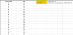
I need to create a drop-down list where the options depend on the value selected in another drop-down list. I used to do this regularly but it has been at least 10 years. Of course, there are probably easier ways to do it now. The way I remember doing it had something to do with the items in the first drop-down being indexed. In the attached image, the user will choose an Opportunity (A, B, C, D or E) in a drop-down in cell D1. That choice would dictate what options for items would be available in the 2nd drop-down in cell D2. As you can see, the number of items will vary by opportunity. Thanks in advance for any help you can provide.

 

[kweaver]

Suggestion: create Name Ranges for each of the Opportunities (e.g., Alist for the As; Blist for the Bs)
Then, in your dependent drop down in D2, make the list selection: =INDIRECT(D1&"list")

 

[bradams]

Suggestion: create Name Ranges for each of the Opportunities (e.g., Alist for the As; Blist for the Bs)
Then, in your dependent drop down in D2, make the list selection: =INDIRECT(D1&"list")

Sorry, I guess I didn't think through my example all the way. The opportunity name won't be incorporated into the item names. Also, the list of opportunities and items will constantly be changing so I couldn't easily define name ranges.

 

[kweaver]

As far as my experience goes, I think the whole idea of dependent drop downs is based on name ranges.

 

[Toadstool]

Hi Bradams,

You can manufacture your dropdown lists from the data then offer them as the dropdown. To avoid lots of blank spaces from unused cells you can also manufacture a reference to the beginning and end of each dropdown then use INDIRECT to only offer those options.
I see you've said there's no content relationship between Opportunity and Item so for Items I've used random words from Shakespeare's "As You Like It".

Bradams.xlsx
	A	B	C	D	E	F	G	H
1	Opportunity	Item		Select Opportunity	D		$G$3:$G$6	$H$3:$H$8
2	A	answerd		Select Item	matron		Opportunity Dropdown	Item Dropdown
3	A	cardinal					A	little
4	A	counterfeit					B	matron
5	A	cranks					C	needy
6	A	distribution					D	obedience
7	A	fair						plague
8	B	harry						poverty
9	B	hollow
10	B	infinite
11	C	king
12	C	lead
13	D	little
14	D	matron
15	D	needy
16	D	obedience
17	D	plague
18	D	poverty
Sheet1

Cell Formulas
Range	Formula
G1	G1	=ADDRESS(ROW($G$3),COLUMN($G$1))&":"&ADDRESS(COUNTIF($G$3:$G$20,"> ")+ROW($G$2),COLUMN($G$3))
H1	H1	=ADDRESS(ROW($H$3),COLUMN($H$1))&":"&ADDRESS(COUNTIF($H$3:$H$20,"> ")+ROW($H$2),COLUMN($H$3))
G3:G18	G3	=INDEX($A$2:$A$9999,MATCH(0,INDEX(COUNTIF($G$2:$G2,$A$2:$A$9999),),0))&""
H3:H18	H3	=IFERROR(INDEX($B$2:$B$9999,AGGREGATE(15,6,ROW($A$2:$A$9999)-ROW($A$1)/($A$2:$A$9999=$E$1),ROW()-ROW($H$2))),"")

Cells with Data Validation
Cell	Allow	Criteria
E1	List	=INDIRECT($G$1)
E2	List	=INDIRECT($H$1)

 

[bradams]

Thank you for putting this together for me! It appears to work but I'm still trying to understand exactly how it works. I'm going to keep working on it tomorrow at the office because it will be easier with dual monitors. For now, I just wanted to say thank you. I may have some more questions tomorrow.

 

[Toadstool]

You're welcome!

 

[kweaver]

Toadstool: beautiful solution to creating the options for the drop downs!!
Would it be save to use UNIQUE(A2:A18) in G3 if running 365?

 

[Toadstool]

Toadstool: beautiful solution to creating the options for the drop downs!!
Would it be save to use UNIQUE(A2:A18) in G3 if running 365?

Thanks!
While I'd like to use UNIQUE and SORT I find most of my Customers are on 2013 or 2016 so I'm staying with 2016 for now... but that means I can't answer your question with any kind of confidence.

btw, I like the constructed range approach for the Data Validation List as it gives a visual confirmation of what list will be used with INDIRECT, but you can also use a similar approach with OFFSET.

Bradams.xlsx
	A	B	C	D	E	F	G	H
1	Opportunity	Item		Select Opportunity	D		Opportunity Dropdown	Item Dropdown
2	A	answerd		Select Item	matron		A	little
3	A	cardinal					B	matron
4	A	counterfeit					C	needy
5	A	cranks					D	obedience
6	A	distribution						plague
7	A	fair						poverty
8	B	harry
9	B	hollow
10	B	infinite
11	C	king
12	C	lead
13	D	little
14	D	matron
15	D	needy
16	D	obedience
17	D	plague
18	D	poverty
19
20
WithOffset

Cell Formulas
Range	Formula
G2:G20	G2	=INDEX($A$2:$A$9999,MATCH(0,INDEX(COUNTIF($G$1:$G1,$A$2:$A$9999),),0))&""
H2:H20	H2	=IFERROR(INDEX($B$2:$B$9999,AGGREGATE(15,6,ROW($A$2:$A$9999)-ROW($A$1)/($A$2:$A$9999=$E$1),ROW()-ROW($H$1))),"")

Cells with Data Validation
Cell	Allow	Criteria
E1	List	=OFFSET($G$2,,,COUNTIF($G$2:$G$20,"> "))
E2	List	=OFFSET($H$2,,,COUNTIF($H$2:$H$20,"> "))