Display a variety of cells in one cell based on multiple variables

[scotchman]

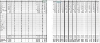
Not sure how to put this but I'll explain what I'm doing. I've created a yearly expenses tracker but in order to have the average of all the months that have gone by I have to edit the variable manually (ex for 3 months gone by =A/3)

I'd like to create a cell for each month gone by and display it in my averages column based on how many months have gone by. So if the March column has an entry in it it displays the average for 3 months. Then once the April column is full it displays the average for 4 months.

I can easily create a bunch of hidden columns but I'm not sure how to pull them to a specific column based on the variables I mentioned. Not even sure if this is possible but I'd love to know how to do it if it is.

Thanks for your help.

 

[Peter_SSs]

Welcome to the MrExcel board!

It is difficult to read your image and in any case we cannot copy from it so there would be a lot of typing to set up a test sheet. I suggest that you make up a small set of dummy data, fill in the results you are asking about manually and post all that with XL2BB
Then explain again in relation to the specific sample data.
(If you have trouble with XL2BB, review the "XL2BB Icons greyed out" link in the 'Known XL2BB issues' section near the top of the XL2BB Instructions page linked above.)

 

[scotchman]

00 Yearly Averages - Template test.xls
	A	B	C	D	E	F	G	H	I	J	K	L	M	N	O
1
2	Item	Jan	%	Feb	%	Mar	%	Total	%	Average		1m average	2m average	3m average
3	Housing	$500.00	14.3%	$1,000.00	26.0%	$1,500.00		$3,000.00	40.8%	$1,000.00		$3,000.00	$1,500.00	$1,000.00
4	Phone	$50.00	1.4%	$100.00	2.6%	$75.00		$225.00	3.1%	$75.00		$225.00	$112.50	$75.00
5	Food	$500.00	14.3%	$550.00	14.3%	$600.00		$1,650.00	22.4%	$550.00		$1,650.00	$825.00	$550.00
6	Clothing	$50.00	1.4%	$75.00	1.9%	$100.00		$225.00	3.1%	$75.00		$225.00	$112.50	$75.00
7	Health	$200.00	5.7%	$300.00	7.8%	$400.00		$900.00	12.2%	$300.00		$900.00	$450.00	$300.00
8	Entertainment	$100.00	2.9%	$200.00	5.2%	$300.00		$600.00	8.2%	$200.00		$600.00	$300.00	$200.00
9	Gas	$250.00	7.1%	$300.00	7.8%	$350.00		$900.00	12.2%	$300.00		$900.00	$450.00	$300.00
10	Car Costs	$550.00	15.7%	$500.00	13.0%	$450.00		$1,500.00	20.4%	$500.00		$1,500.00	$750.00	$500.00
11	Bank Fees/Loans	$30.00	0.9%	$25.00	0.6%	$20.00		$75.00	1.0%	$25.00		$75.00	$37.50	$25.00
12	Tools	$50.00	1.4%	$100.00	2.6%	$150.00		$300.00	4.1%	$100.00		$300.00	$150.00	$100.00
13	Misc	$50.00	1.4%	$50.00	1.3%	$50.00		$150.00	2.0%	$50.00		$150.00	$75.00	$50.00
14
15	Work Income	$3,000.00	85.7%	$3,500.00	90.9%			$6,500.00	88.4%	$541.67		$6,500.00	$3,250.00	$2,166.67
16	Music Income	$200.00	5.7%	$300.00	7.8%			$500.00	6.8%	$41.67		$500.00	$250.00	$166.67
17	Govt Income	$300.00	8.6%	$50.00	1.3%			$350.00	4.8%	$29.17		$350.00	$175.00	$116.67
18
19	Total Income	$3,500.00		$3,850.00				$7,350.00		$612.50		$7,350.00	$3,675.00	$2,450.00
20	Total Expenses	$2,330.00		$3,200.00				$9,525.00		$793.75		$9,525.00	$4,762.50	$3,175.00
21	Surplus	$1,170.00		$650.00				-$2,175.00		-$181.25		-$2,175.00	-$1,087.50	-$725.00
22
23
Sheet1

Cell Formulas
Range	Formula
L3:L21	L3	=IF(H3="","",H3)
M3:M21	M3	=IF(H3="","",H3/2)
N3:N21	N3	=IF(H3="","",H3/3)
C3:C13,C15:C17	C3	=IF($B$19="","",B3/$B$19)
E3:E13,E15:E17	E3	=IF($D$19="","",D3/$D$19)
G3:G13,G15:G17	G3	=IF($F$19="","",F3/$F$19)
I3:I13,I15:I18	I3	=IF(H3="","",H3/$H$19)
B19,H19,F19,D19	B19	=IF(B15="","",B15+B16+B17)
B20,H20	B20	=IF(B19="","",SUM(B3:B13))
B21,H21	B21	=IF(B19="","",B19-B20)
D20,F20	D20	=IF(D15="","",SUM(D3:D13))
D21,F21	D21	=IF(D15="","",D19-D20)
H3:H17	H3	=IF(B3="","",B3+D3+F3)
H18	H18	=IF(B18="","",B18+D18+F18+#REF!+#REF!+#REF!+#REF!+#REF!+#REF!+#REF!+#REF!+#REF!)
J3:J14	J3	=N3
J15:J21	J15	=IF(H15="","",H15/12)
J22:J23	J22	=IF(H22="","",H22/4)

 

[scotchman]

Sorry I'll simplify it a bit.

00 Yearly Averages - Template test.xls
	G
6	$75.00
Sheet1

Cell Formulas
Range	Formula
G6	G6	=K6

 

[scotchman]

Ugh whoops sorry here. I'm a n00b excuse my mistakes.

00 Yearly Averages - Template test.xls
	A	B	C	D	E	F	G	H	I	J	K	L
1
2	Item	Jan	Feb	Mar	Total	%	Average		1m average	2m average	3m average
3	Housing	$500.00	$1,000.00	$1,500.00	$3,000.00	25.0%	$1,000.00		$500.00	$750.00	$1,000.00
4	Phone	$50.00	$100.00	$75.00	$225.00	1.9%	$75.00		$50.00	$75.00	$75.00
5	Food	$500.00	$550.00	$600.00	$1,650.00	13.8%	$550.00		$500.00	$525.00	$550.00
6	Clothing	$50.00	$75.00	$100.00	$225.00	1.9%	$75.00		$50.00	$62.50	$75.00
7	Health	$200.00	$300.00	$400.00	$900.00	7.5%	$300.00		$200.00	$250.00	$300.00
8	Entertainment	$100.00	$200.00	$300.00	$600.00	5.0%	$200.00		$100.00	$150.00	$200.00
9	Gas	$250.00	$300.00	$350.00	$900.00	7.5%	$300.00		$250.00	$275.00	$300.00
10	Car Costs	$550.00	$500.00	$450.00	$1,500.00	12.5%	$500.00		$550.00	$525.00	$500.00
11	Bank Fees/Loans	$30.00	$25.00	$20.00	$75.00	0.6%	$25.00		$30.00	$27.50	$25.00
12	Tools	$50.00	$100.00	$150.00	$300.00	2.5%	$100.00		$50.00	$75.00	$100.00
13	Misc	$50.00	$50.00	$50.00	$150.00	1.3%	$50.00		$50.00	$50.00	$50.00
14							$0.00
15	Work Income	$3,000.00	$3,500.00	$4,000.00	$10,500.00	87.5%	$875.00		$3,000.00	$3,250.00	$3,500.00
16	Music Income	$200.00	$300.00	$400.00	$900.00	7.5%	$75.00		$200.00	$250.00	$300.00
17	Govt Income	$300.00	$100.00	$200.00	$600.00	5.0%	$50.00		$300.00	$200.00	$200.00
18
19	Total Income	$3,500.00	$3,900.00	$4,600.00	$12,000.00		$1,000.00		$3,500.00	$3,700.00	$4,000.00
20	Total Expenses	$2,330.00	$3,200.00	$3,995.00	$9,525.00		$793.75		$2,330.00	$2,765.00	$3,175.00
21	Surplus	$1,170.00	$700.00	$605.00	$2,475.00		$206.25		$1,170.00	$935.00	$825.00
22
Sheet1

Cell Formulas
Range	Formula
E3:E13,E15:E17	E3	=B3+C3+D3
F3:F13,F15:F18	F3	=IF(E3="","",E3/$E$19)
I3:I13,I19:I21,I15:I17	I3	=B3
J3:J13,J19:J21,J15:J17	J3	=(B3+C3)/2
K3:K13,K19:K21,K15:K17	K3	=(B3+C3+D3)/3
E18	E18	=IF(B18="","",B18+C18+D18+#REF!+#REF!+#REF!+#REF!+#REF!+#REF!+#REF!+#REF!+#REF!)
B19:E19	B19	=IF(B15="","",B15+B16+B17)
B20,E20	B20	=IF(B19="","",SUM(B3:B13))
C20:D20	C20	=IF(C15="","",SUM(C3:C13))
B21,E21	B21	=IF(B19="","",B19-B20)
C21:D21	C21	=IF(C15="","",C19-C20)
G3:G14	G3	=K3
G15:G21	G15	=IF(E15="","",E15/12)
G22	G22	=IF(E22="","",E22/4)

 

[scotchman]

So basically I want column G to display either column I J or K depending on how much of the table from A:D is filled out. So if Jan and Feb are filled it, it displays the 2 month average, if march is filled in it displays the 3 month average, and so on.

 

[Peter_SSs]

Thanks for getting XL2BB up and running.

I have altered some of the data to demonstrate

I am not sure if you mean this ..

24 11 11.xlsm
	G	H	I	J	K
2	Average		1m average	2m average	3m average
3	1000		500	750	1000
4	50		50
5	500		500
6	50		50
7	300		200	250	300
8	150		100	150
9	275		250	275
Average

Cell Formulas
Range	Formula
J3,J7:J9	J3	=(B3+C3)/2
K3,K7	K3	=(B3+C3+D3)/3
I3:I9	I3	=B3
G3:G9	G3	=IFNA(LOOKUP(9^9,I3:K3),"")

.. or this

24 11 11.xlsm
	B	C	D	E		G
2	Jan	Feb	Mar	Total		Average
3	500	1000	1500	3000		1000
4	50			50		50
5	500			500		500
6	50	75		125		62.5
7	200	300		500		250
8	100	200	300	600		200
Average (2)

Cell Formulas
Range	Formula
E3:E8	E3	=B3+C3+D3
G3:G8	G3	=AVERAGE(B3:D3)

.. or something else?

 

[scotchman]

Here I'll post 3 sheets as if it was progressing through the months.

Edit: ignore this reply I made a mistake and didn't find the edit button until after I posted the following post

 

[scotchman]

Whoops I didn't post the first one, let me try again.

00 Yearly Averages - Template test.xls
	A	B	C	D	E	F	G
2	Item	Jan	Feb	Mar	Total	%	Average
3	Housing	$500.00			$500.00	14.3%	$500.00
4	Phone	$50.00			$50.00	1.4%	$50.00
5	Food	$500.00			$500.00	14.3%	$500.00
6	Clothing	$50.00			$50.00	1.4%	$50.00
7	Health	$200.00			$200.00	5.7%	$200.00
8	Entertainment	$100.00			$100.00	2.9%	$100.00
9	Gas	$250.00			$250.00	7.1%	$250.00
10	Car Costs	$550.00			$550.00	15.7%	$550.00
11	Bank Fees/Loans	$30.00			$30.00	0.9%	$30.00
12	Tools	$50.00			$50.00	1.4%	$50.00
13	Misc	$50.00			$50.00	1.4%	$50.00
14
15	Work Income	$3,000.00			$3,000.00	85.7%	$3,000.00
16	Music Income	$200.00			$200.00	5.7%	$200.00
17	Govt Income	$300.00			$300.00	8.6%	$300.00
18
19	Total Income	$3,500.00			$3,500.00		$3,500.00
20	Total Expenses	$2,330.00			$2,330.00		$2,330.00
21	Surplus	$1,170.00			$1,170.00		$1,170.00
Sheet1

Cell Formulas
Range	Formula
E3:E13,E15:E17	E3	=B3+C3+D3
F3:F13,F15:F18	F3	=IF(E3="","",E3/$E$19)
G3:G13,G19:G21,G15:G17	G3	=I3
B19,E19	B19	=IF(B15="","",B15+B16+B17)
B20,E20	B20	=IF(B19="","",SUM(B3:B13))
B21,E21	B21	=IF(B19="","",B19-B20)
E18	E18	=IF(B18="","",B18+C18+D18+#REF!+#REF!+#REF!+#REF!+#REF!+#REF!+#REF!+#REF!+#REF!)

00 Yearly Averages - Template test.xls
	A	B	C	D	E	F	G
24	Item	Jan	Feb	Mar	Total	%	Average
25	Housing	$500.00	$1,000.00		$1,500.00	42.9%	$750.00
26	Phone	$50.00	$100.00		$150.00	4.3%	$75.00
27	Food	$500.00	$550.00		$1,050.00	30.0%	$525.00
28	Clothing	$50.00	$75.00		$125.00	3.6%	$62.50
29	Health	$200.00	$300.00		$500.00	14.3%	$250.00
30	Entertainment	$100.00	$200.00		$300.00	8.6%	$150.00
31	Gas	$250.00	$300.00		$550.00	15.7%	$275.00
32	Car Costs	$550.00	$500.00		$1,050.00	30.0%	$525.00
33	Bank Fees/Loans	$30.00	$25.00		$55.00	1.6%	$27.50
34	Tools	$50.00	$100.00		$150.00	4.3%	$75.00
35	Misc	$50.00	$50.00		$100.00	2.9%	$50.00
36
37	Work Income	$3,000.00	$3,500.00		$6,500.00	185.7%	$3,250.00
38	Music Income	$200.00	$300.00		$500.00	14.3%	$250.00
39	Govt Income	$300.00	$100.00		$400.00	11.4%	$200.00
40
41	Total Income	$3,500.00	$3,900.00		$7,400.00		$3,700.00
42	Total Expenses	$2,330.00	$3,200.00		$5,530.00		$2,765.00
43	Surplus	$1,170.00	$700.00		$1,870.00		$935.00
Sheet1

Cell Formulas
Range	Formula
E25:E35,E37:E39	E25	=B25+C25+D25
F25:F35,F37:F40	F25	=IF(E25="","",E25/$E$19)
G25:G35,G41:G43,G37:G39	G25	=(B25+C25)/2
B41:C41,E41	B41	=IF(B37="","",B37+B38+B39)
B42,E42	B42	=IF(B41="","",SUM(B25:B35))
C42	C42	=IF(C37="","",SUM(C25:C35))
B43,E43	B43	=IF(B41="","",B41-B42)
C43	C43	=IF(C37="","",C41-C42)
E40	E40	=IF(B40="","",B40+C40+D40+#REF!+#REF!+#REF!+#REF!+#REF!+#REF!+#REF!+#REF!+#REF!)

00 Yearly Averages - Template test.xls
	A	B	C	D	E	F	G
45	Item	Jan	Feb	Mar	Total	%	Average
46	Housing	$500.00	$1,000.00	$1,500.00	$3,000.00	85.7%	$1,000.00
47	Phone	$50.00	$100.00	$75.00	$225.00	6.4%	$75.00
48	Food	$500.00	$550.00	$600.00	$1,650.00	47.1%	$550.00
49	Clothing	$50.00	$75.00	$100.00	$225.00	6.4%	$75.00
50	Health	$200.00	$300.00	$400.00	$900.00	25.7%	$300.00
51	Entertainment	$100.00	$200.00	$300.00	$600.00	17.1%	$200.00
52	Gas	$250.00	$300.00	$350.00	$900.00	25.7%	$300.00
53	Car Costs	$550.00	$500.00	$450.00	$1,500.00	42.9%	$500.00
54	Bank Fees/Loans	$30.00	$25.00	$20.00	$75.00	2.1%	$25.00
55	Tools	$50.00	$100.00	$150.00	$300.00	8.6%	$100.00
56	Misc	$50.00	$50.00	$50.00	$150.00	4.3%	$50.00
57							$0.00
58	Work Income	$3,000.00	$3,500.00	$4,000.00	$10,500.00	300.0%	$3,500.00
59	Music Income	$200.00	$300.00	$400.00	$900.00	25.7%	$300.00
60	Govt Income	$300.00	$100.00	$200.00	$600.00	17.1%	$200.00
61
62	Total Income	$3,500.00	$3,900.00	$4,600.00	$12,000.00		$4,000.00
63	Total Expenses	$2,330.00	$3,200.00	$3,995.00	$9,525.00		$3,175.00
64	Surplus	$1,170.00	$700.00	$605.00	$2,475.00		$825.00
Sheet1

Cell Formulas
Range	Formula
E46:E56,E58:E60	E46	=B46+C46+D46
F46:F56,F58:F61	F46	=IF(E46="","",E46/$E$19)
G62:G64,G46:G60	G46	=(B25+C25+D46)/3
E61	E61	=IF(B61="","",B61+C61+D61+#REF!+#REF!+#REF!+#REF!+#REF!+#REF!+#REF!+#REF!+#REF!)
B62:E62	B62	=IF(B58="","",B58+B59+B60)
B63,E63	B63	=IF(B62="","",SUM(B46:B56))
C63:D63	C63	=IF(C58="","",SUM(C46:C56))
B64,E64	B64	=IF(B62="","",B62-B63)
C64:D64	C64	=IF(C58="","",C62-C63)

Again, its the averages column I want to update based on which month we're in. I don't want to have to edit the divisor based on which month we're in, I want it to automatically change the divisor.

 

[Peter_SSs]

Again, its the averages column I want to update ..

I'm not sure that you tried the suggestions that I made before, particularly the second one?

Here I have used the same formula all the way down column G. The results are the same as those from your 3 different formulas.
(The AVERAGE function knows to sum the values and divide by the correct number, ignoring empty cells )

24 11 11.xlsm
	A	B	C	D	E		G
1
2	Item	Jan	Feb	Mar	Total		Average
3	Housing	$500.00			$500.00		$500.00
4	Phone	$50.00			$50.00		$50.00
5	Food	$500.00			$500.00		$500.00
6	Clothing	$50.00			$50.00		$50.00
7	Health	$200.00			$200.00		$200.00
8	Entertainment	$100.00			$100.00		$100.00
9	Gas	$250.00			$250.00		$250.00
10	Car Costs	$550.00			$550.00		$550.00
11	Bank Fees/Loans	$30.00			$30.00		$30.00
12	Tools	$50.00			$50.00		$50.00
13	Misc	$50.00			$50.00		$50.00
14
15	Work Income	$3,000.00			$3,000.00		$3,000.00
16	Music Income	$200.00			$200.00		$200.00
17	Govt Income	$300.00			$300.00		$300.00
18
19	Total Income	$3,500.00			$3,500.00		$3,500.00
20	Total Expenses	$2,330.00			$2,330.00		$2,330.00
21	Surplus	$1,170.00			$1,170.00		$1,170.00
22
23
24	Item	Jan	Feb	Mar	Total		Average
25	Housing	$500.00	$1,000.00		$1,500.00		$750.00
26	Phone	$50.00	$100.00		$150.00		$75.00
27	Food	$500.00	$550.00		$1,050.00		$525.00
28	Clothing	$50.00	$75.00		$125.00		$62.50
29	Health	$200.00	$300.00		$500.00		$250.00
30	Entertainment	$100.00	$200.00		$300.00		$150.00
31	Gas	$250.00	$300.00		$550.00		$275.00
32	Car Costs	$550.00	$500.00		$1,050.00		$525.00
33	Bank Fees/Loans	$30.00	$25.00		$55.00		$27.50
34	Tools	$50.00	$100.00		$150.00		$75.00
35	Misc	$50.00	$50.00		$100.00		$50.00
36
37	Work Income	$3,000.00	$3,500.00		$6,500.00		$3,250.00
38	Music Income	$200.00	$300.00		$500.00		$250.00
39	Govt Income	$300.00	$100.00		$400.00		$200.00
40
41	Total Income	$3,500.00	$3,900.00		$7,400.00		$3,700.00
42	Total Expenses	$2,330.00	$3,200.00		$5,530.00		$2,765.00
43	Surplus	$1,170.00	$700.00		$1,870.00		$935.00
44
45	Item	Jan	Feb	Mar	Total		Average
46	Housing	$500.00	$1,000.00	$1,500.00	$3,000.00		$1,000.00
47	Phone	$50.00	$100.00	$75.00	$225.00		$75.00
48	Food	$500.00	$550.00	$600.00	$1,650.00		$550.00
49	Clothing	$50.00	$75.00	$100.00	$225.00		$75.00
50	Health	$200.00	$300.00	$400.00	$900.00		$300.00
51	Entertainment	$100.00	$200.00	$300.00	$600.00		$200.00
52	Gas	$250.00	$300.00	$350.00	$900.00		$300.00
53	Car Costs	$550.00	$500.00	$450.00	$1,500.00		$500.00
54	Bank Fees/Loans	$30.00	$25.00	$20.00	$75.00		$25.00
55	Tools	$50.00	$100.00	$150.00	$300.00		$100.00
56	Misc	$50.00	$50.00	$50.00	$150.00		$50.00
57
58	Work Income	$3,000.00	$3,500.00	$4,000.00	$10,500.00		$3,500.00
59	Music Income	$200.00	$300.00	$400.00	$900.00		$300.00
60	Govt Income	$300.00	$100.00	$200.00	$600.00		$200.00
61
62	Total Income	$3,500.00	$3,900.00	$4,600.00	$12,000.00		$4,000.00
63	Total Expenses	$2,330.00	$3,200.00	$3,995.00	$9,525.00		$3,175.00
64	Surplus	$1,170.00	$700.00	$605.00	$2,475.00		$825.00
Average (3)

Cell Formulas
Range	Formula
G3:G13,G62:G64,G58:G60,G46:G56,G41:G43,G37:G39,G25:G35,G19:G21,G15:G17	G3	=AVERAGE(B3:D3)

.. and if you want to use the same formula without having to skip the blank rows, you can use this modification.

24 11 11.xlsm
	B	C	D	E			H
1
2	Jan	Feb	Mar	Total			Average
3	$500.00			$500.00			$500.00
4	$50.00			$50.00			$50.00
5	$500.00			$500.00			$500.00
6	$50.00			$50.00			$50.00
7	$200.00			$200.00			$200.00
8	$100.00			$100.00			$100.00
9	$250.00			$250.00			$250.00
10	$550.00			$550.00			$550.00
11	$30.00			$30.00			$30.00
12	$50.00			$50.00			$50.00
13	$50.00			$50.00			$50.00
14
15	$3,000.00			$3,000.00			$3,000.00
16	$200.00			$200.00			$200.00
17	$300.00			$300.00			$300.00
18
19	$3,500.00			$3,500.00			$3,500.00
20	$2,330.00			$2,330.00			$2,330.00
21	$1,170.00			$1,170.00			$1,170.00
22
23
24	Jan	Feb	Mar	Total
25	$500.00	$1,000.00		$1,500.00			$750.00
26	$50.00	$100.00		$150.00			$75.00
27	$500.00	$550.00		$1,050.00			$525.00
28	$50.00	$75.00		$125.00			$62.50
29	$200.00	$300.00		$500.00			$250.00
30	$100.00	$200.00		$300.00			$150.00
31	$250.00	$300.00		$550.00			$275.00
32	$550.00	$500.00		$1,050.00			$525.00
33	$30.00	$25.00		$55.00			$27.50
34	$50.00	$100.00		$150.00			$75.00
35	$50.00	$50.00		$100.00			$50.00
36
37	$3,000.00	$3,500.00		$6,500.00			$3,250.00
Average (5)

Cell Formulas
Range	Formula
H3:H37	H3	=IFERROR(AVERAGE(B3:D3),"")