DAX: Double or Nested COUNTX() & SUMX()

[luuk]

Hello,

For certain products, we have a variable pricing concept and through a power pivot table we're trying to determine - by product (row) - for every sales price (value) the mean, deviation from mean and standard deviation. We use measures in the pivot table to come to the standard deviation - per product. As we need to be able to filter within the pivot table. We assume that we lose analytical capabilities if we move these fields as calculated columns in the data model.

We are stuck with a double, or nested, COUNTX & SUMX.

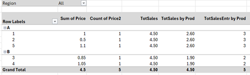
Refer to the example below. Assume we have product A with 5 sales entries. We need (1) the mean price for this product, (2) for every of the 5 sales entries the deviation of the sales price from the mean, and (3) for every of the 5 sales entries the standard deviation. To determine the mean, you need the total price column (4,50) divided by the number of sales items (5). To determine the deviation per sales entry, you need both values available on every row.

'Measure 1' is a stepping-stone to get to the mean. We use DAX formula =CALCULATE(COUNTAX(Table3, Table3[Counter]), ALL(Table3[ID])). It sums up the number of items in scope, based on the Counter column, and set the result (5) in every line. This works fine.

Another summarization is needed. The example in 'measure 2' is significantly simplified.

For 'measure 2' we want to summarize the values of 'measure 1' and put the outcome (25) in every line. We used DAX formula =CALCULATE(COUNTAX(Table3, Table3[Measure 1]), ALL(Table3[ID])). This does not work. The outcome is that the 'measure 1' value (5) is put in 'measure 2' in every line. It seems that a measure with COUNTX on a measure with COUNTX is not working. The same problem applies with a measure with SUMX on a measure with a SUMX. Then, the output is always 0.00.

Is it correct that a COUNTX on a COUNTX, and a SUMX on a SUMX is not possible?

Are there alternative ways how to create a pivot table measure that sets the values as per the 'measure 2' of the example?

Thank you,
Luuk

 

[Matt Allington]

It is quite possible that the approach you are taking is more difficult than it needs to be, but I can't be sure.

1. What is the counter that I can see in the first table? Is it always 1? If so, you don't need it.
2. Do you have a star schema? If not, you should set that up first. https://exceleratorbi.com.au/the-optimal-shape-for-power-pivot-data/

post back a sample workbook after doing these things and I will take a look

 

[luuk]

Hi Matt, all,

To answer your questions:
1. The counter is there to simplify the example. In reality it is the counter of the Sales ID. (In the below example the counter is by Price ).
2. The dataset used is an extract from our general ledger, but the calculation of the standard deviation is based on a couple of columns. The real world example will likely have the products in a 2nd table but I don't really see a need to adjust the data model.

I am not allowed to upload the workbook, but as the problem can be shown in a straightforward example, hopefully the below is enough?

I've simplified / anonymized the table. You see the Sales ID, the price, the region (not used now, but expected in the final model), and the product. Total sales is 4.50 based on 5 transactions.

To calculate the standard deviation, I use a single pivot table. For my problem, I've split it to two.

First, the transactions (COUNTAX) example - see below:
- There are 3 transactions for product A, and 2 Transactions for product B.
- The Sales ID (transactions) is in column B.
- Columns Price (C) and Count of Price2 (D) come from the dataset.
- The measure in column E calculates the total of the Sales ID (5) and puts it on every row. (The column total is wrong, but that is okay.)
- The measure in column F calculates the total of the Sales ID per product. (The column total is wrong, but that is okay.)
- The measure in column G must calculate the total of column F. Here the problem occurs.

The formula for column F: =CALCULATE(COUNTAX(Table1, Table1[Price]), All(Table1[ID]))
The formula for column G: =CALCULATE(COUNTAX(Table1, Table1[TotSalesEntries by Prod]), ALL(Table1[ID]))

The outcome in column G is not correct. For product A there are 3 sales ID and for product B there are 2 sales ID. The expected outcome in column G is 9 for product A (3 sales ID * 3.00 (column F)) and 4.00 for product B (2 sales ID * 2.00 (column F)). Just like the measure for column F.

Second, the price (SUMX) example - see below:
- The measure in column E calculates the total of the Sales (4.50) and puts it on every row. (The column total is wrong, but that is okay.)
- The measure in column F calculates the total of the Sales per product. (The column total is wrong, but that is okay.)
- The measure in column G must calculate the total of column F. The same problem occurs.

The formula for column F: =CALCULATE(SUMX(Table1, Table1[Sum of Price]), ALL(Table1[ID]))
The formula for column G: =CALCULATE(SUMX(Table1,Table1[TotSales by Prod]), ALL(Table1[ID]))

The outcome in column G is not correct. For product A the total sales is 2.60 and for product B it is 1.90. The expected outcome in column G is 7.80 for product A (3 sales ID * 2.60 (column F) and 3.80 for product B (2 sales ID * 1.90 (column F)). Just like the measure for column F.

It appears that the first COUNTAX and SUMX (columns E and F) work well. The outcome is as expected. But that a COUNTAX or SUMX on a measure (column F) that contains already a COUNTAX or SUMX is confusing for the pivot table.

Hope this clarifies. Thank you.
Luuk

 

[Matt Allington]

The outcome in column G is not correct. For product A there are 3 sales ID and for product B there are 2 sales ID. The expected outcome in column G is 9 for product A (3 sales ID * 3.00 (column F))

I don't understand why you are treating "3 sales ID" and Column F differently. They are the same number based on the same calculation from what I can see. Are you saying they can be different? If so, I suggest you adjust your test data to reflect that and repost.

Second, the price (SUMX) example - see below:
- The measure in column E calculates the total of the Sales (4.50) and puts it on every row. (The column total is wrong, but that is okay.)

The column total looks right to me. It is the total of all sales = $4.50. What is wrong with it?

The formula for column F: =CALCULATE(SUMX(Table1, Table1[Sum of Price]), ALL(Table1[ID]))

As I mentioned earlier

Do you have a star schema? If not, you should set that up first. The Optimal Shape for Power BI Data

You are unlikely to reliably solve the issue until you have a stars schema. Anytime you are using CALCULATE to manipulate filtering behaviour, you should do it over a dimension table, not a fact table. This is because of the way Power BI compresses and stores data in the database.

 

[luuk]

Hi Matt, all,

The outcomes of columns E and F are correct. The issue is with column G.

Perhaps the reference back to my initial post with my 1 - 5 - 25 measures will clarify.

The objective of both columns F is to calculate the total per product. For price this is 2.60 for product A and 1.90 for product B. And this is fine. For column G, the formula follows the same syntax but it now takes the measure in column F [TotSales by Prod]. In column F for product A you have 3 lines with 2.60: The total of 7.80 (3 items of 2.60) must be set in each line of column G. For Product B you have 2 lines with 1.90: The total of 3.80 (2 items of 1.90) must be set in each line of column G.

I have been playing with the ALL() filters and I agree that the use of the filters trigger the wrong result of column G.

I did read your blog on the shape of my data set. I am not sure I understand the "up hill" and "down hill" idea, but what you're saying is that if I change the Product in my main dataset to ProductKey and create a look-up table with ProductKey and Product, the filtering of my nested SUMX and COUNTAX formulas are easier.

I will give it a go.

Thank you, kind regards, Luuk

 

[Matt Allington]

Have you deployed the Star Schema yet? I can't help you until you have done that.

 

[luuk]

Hi Matt,

I struggled what benefit your Star Schema would give me. Especially, as the 4-column dataset comes directly from the ledger and it seems strange that I would need to split it up to make it work. Instead, I focused on the filters, and with some help of ChatGPT , I build an inner measure and an outer measure that uses the inner measure to perform the calculation. That now works. You see that that outer measure nicely sums up the inner measure. This concept is exactly what I need to build up subsequent measures to calculate the volatility (standard deviation) of the sales per product.

InnerSumPrice = CALCULATE(SUM(Table1[Price]), ALLEXCEPT(Table1, Table1[Product]))
OuterCountPrice = CALCULATE(SUMX(VALUES(Table1[ID]), [InnerSumPrice]), ALLEXCEPT(Table1, Table1[Product]))
OuterCountPriceNested =CALCULATE(SUMX(VALUES(Table1[ID]), CALCULATE(SUM(Table1[Price]), ALLEXCEPT(Table1, Table1[Product]))), ALLEXCEPT(Table1, Table1[Product]))

Thanks for pointing me to the filters.

Kind regards, Luuk