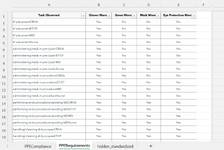
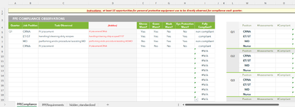
cross-referencing between 2 worksheets

[JEK]

Quarter	Job Position	Observed Task	[hidden]	Gloves Worn?	Gown Worn?	Mask Worn?	Eye Protection Worn?	Compliant?
[list: Q1; Q2; Q3; Q4]	[list: CRNA; ET/ST; MD; Nurse]	[list: task1; task2; task3; task4; task5; task6]	[formula: =C2&B2]	[list: Yes; No]	[list: Yes; No]	[list: Yes; No]	[list: Yes; No]	[forumla to populate "compliant", "non-compliant", or blank]

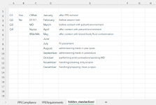
The above is an example of a compliance tool that will allow managers to document workplace observations. Columns A thru G will be standardized by using data validation lists (standardized lists on on a seperate, hidden worksheet within the same workbook). I have create a seperate worksheet, within the same workbook, with a list of each position type, performing each different job task, and what PPE is required, using "Yes" for any required ppe.
I need column I to refer to this seperate worksheet2 when determining compliance, which it is currently doing with the formula provided below- however, if the employee is wearing additional ppe that is not required, this should not affect compliance (only lack of required items result in non-compliance); the formula below does not do this. The formula also returns "N/A" on blank rows, therefore I need to work in how to return a blank in I5 if D5 is blank.

I am beginner-level so there may be many better formulas to use for my needs, but currently this formula is used in I5 ("Compliant?" column):

=IF(
AND(
IF(ISBLANK(VLOOKUP($E5, PPERequirements!$A:$E, MATCH("Gloves Worn?", PPERequirements!$1:$1, 0), FALSE)), FALSE, VLOOKUP($E5, PPERequirements!$A:$E, MATCH("Gloves Worn?", PPERequirements!$1:$1, 0), FALSE) = $F5),
IF(ISBLANK(VLOOKUP($E5, PPERequirements!$A:$E, MATCH("Gown Worn?", PPERequirements!$1:$1, 0), FALSE)), FALSE, VLOOKUP($E5, PPERequirements!$A:$E, MATCH("Gown Worn?", PPERequirements!$1:$1, 0), FALSE) = $G5),
IF(ISBLANK(VLOOKUP($E5, PPERequirements!$A:$E, MATCH("Mask Worn?", PPERequirements!$1:$1, 0), FALSE)), FALSE, VLOOKUP($E5, PPERequirements!$A:$E, MATCH("Mask Worn?", PPERequirements!$1:$1, 0), FALSE) = $H5),
IF(ISBLANK(VLOOKUP($E5, PPERequirements!$A:$E, MATCH("Eye Protection Worn?", PPERequirements!$1:$1, 0), FALSE)), FALSE, VLOOKUP($E5, PPERequirements!$A:$E, MATCH("Eye Protection Worn?", PPERequirements!$1:$1, 0), FALSE) = $I5)
),
"compliant",
"non-compliant"
)

 

[Sam_D_Ben]

Something like this,

=IF(ISBLANK(D5),"",IF(OR(VLOOKUP($E5,PPERequirements!$A:$E,MATCH("Gloves Worn?",PPERequirements!$1:$1,0),FALSE)<>$F5,VLOOKUP($E5,PPERequirements!$A:$E,MATCH("Gown Worn?",PPERequirements!$1:$1,0),FALSE)<>$G5,VLOOKUP($E5,PPERequirements!$A:$E,MATCH("Mask Worn?",PPERequirements!$1:$1,0),FALSE)<>$H5,VLOOKUP($E5,PPERequirements!$A:$E,MATCH("Eye Protection Worn?",PPERequirements!$1:$1,0),FALSE)<>$I5),"non-compliant","compliant")))

Or

=IF(ISBLANK(D5), "", IF(COUNTIFS(PPERequirements!$A:$A, $E5, PPERequirements!$B:$B, $F5, PPERequirements!$C:$C, $G5, PPERequirements!$D:$D, $H5, PPERequirements!$E:$E, $I5) > 0, "compliant", "non-compliant"))

 

[JEK]

Thank you for your reply! However, its still not working
When I use the first formula you provided it produces N/A. I tried a few adjustments to see if I could tell what the issue was but go no change when the following items were adjusted, one at a time, and returned prior to the sequential adjustment:
No change in forumlated when:
- row is blank
- boxes are filled as compliant
- cells are formatted as "general"
- cells are formatted as "text"
- Instead of "No" to mark items not required on PPERequirements chart, blank is used
- "No" used to mark items not required on PPERequirements chart
- row 5 of PPERequirements chart is compliant/matching data in row 5 of compliance worksheet

The second formula provided above produces "non-compliant" - same results when troubleshooting, in that there is no change from "non-compliant".
I feel like I'm missing something dumb that I should probably know because I've tried so many different formulas and have tried to get answers from 2 different AI programs, as well.

 

[Sam_D_Ben]

Hi How are you! I like to to know, the above example you provided/ is that the actual format of the orginal one, AND can i see the sample "PPERequirements!" sheet AND the example table look like some query output, AND all i did was simply adjusted the structure of your formula without altering its functionality. Maybe if you can provide more samples, i guess we can try, TY

 

[Alex Blakenburg]

Also your words say that your formula is in Column I but the formula you pasted in uses columns G to I as the Yes/No values which means the formula would eed to be in Column J. The test for D5 being blank indicates that the Lookup value used is in Column D but the formula uses E.
Please show an image that includes the row and column references to clarify the position of your data.
Also an image of the Lookup Table including the row and column references. (Do the column headings match ?)

 

[JEK]

Sam, I used the "copy to clipboard" button on your formula box, and pasted that into cell I5.
Alex, column I5 will not have a yes/no value, it will (hopefully) populate with the "compliant" or "non-compliant". I'm not 100% certain I'm understanding your Column D/Column E statement but I just tried replacing "$E5" in the 1st formula with "$D5" and had no change in results.
I appreciate y'alls comments. I have taken a screenshot of all 3 worksheets referenced - including the one for data validation just in case.

 

[Alex Blakenburg]

That is consistent with your data in the OP but not consistent with the formula you provided, @Sam_D_Ben also used the formula as the driver for what cells to use.

See if something like this works for you:

=LET(dataHdg,$E$1:$H$1,
dataHdgVal,LEFT(dataHdg,LEN(dataHdg)-1),
dataRow,$E5:$H5,
lkValues,INDEX(PPERequirements!$A:$E,MATCH($D5,PPERequirements!$A:$A,0),MATCH(dataHdgVal,PPERequirements!$1:$1,0)),
IF(SUM((lkValues=dataRow)+(lkValues<>"Yes")*(lkValues<>dataRow))=COLUMNS(dataHdg),"Compliant","Non-Compliant"))

 

[JEK]

Thank you both very much for your advice. I have finally gotten a formula that works! I got rid of column D all together (this was only added due to input from other sources). I will post below if curious. Have a great day

=IF(B5="","",
IF(AND(
IF(INDEX('PPERequirements'!C:C, MATCH(B5&C5, 'PPERequirements'!A:A&'PPERequirements'!B:B, 0))="Yes", D5="Yes", TRUE),
IF(INDEX('PPERequirements'!D:D, MATCH(B5&C5, 'PPERequirements'!A:A&'PPERequirements'!B:B, 0))="Yes", E5="Yes", TRUE),
IF(INDEX('PPERequirements'!E:E, MATCH(B5&C5, 'PPERequirements'!A:A&'PPERequirements'!B:B, 0))="Yes", F5="Yes", TRUE),
IF(INDEX('PPERequirements'!F:F, MATCH(B5&C5, 'PPERequirements'!A:A&'PPERequirements'!B:B, 0))="Yes", G5="Yes", TRUE)
), "Compliant", "Non-Compliant"))

 

[Alex Blakenburg]

Thanks for letting us know. Glad you found something that worked for you.