Create Variable Interest Rate Amortization Schedule using Dynamic Arrays

AEAA

New Member
Joined
Apr 12, 2022
Messages
35
Office Version
  1. 365
  2. 2021
Platform
  1. Windows
Hello All,

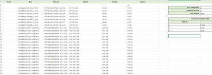
I've been struggling a lot with what seems to be a quite simple calculation. I am trying to make an Amortization Schedule for a Mortgage with variable interest rate. And using standard cell by cell formulas it can be easily done. (See attachment as example).

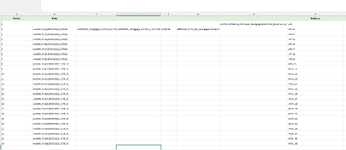
So I basically first start by calculating my monthly payment using PMT and the initial loan value. Then I can calculate the interest and the installment and subtract that from the initial loan to get the principal balance of the current month. Then I can just refer to that value in the row below and drag the formula all the way down. However, If I try to do exactly the same using Dynamic Ranges/formulas, it sees it as a circular reference simply since within the array there is the previous value. Is there any workaround for this? I need this to be a dynamic range. Also attached below.

I managed to use everything dynamic:

=-PMT(EIR_Mortgage_Monthly/12;Total_Payments_Mortgage-Month+1;P2:P25)

P2:P25 should be the Array of the end balance but thats where the Dynamic reference falls apart.

End Balance formula: Effective_Principal_Mortgage-SCAN(0;Installments_Monthly;LAMBDA(a;b;a+b))

Any help would be appreciated. Thanks
 

Attachments

  • Example.PNG
    Example.PNG
    76.5 KB · Views: 9
  • Example_Dynamic.PNG
    Example_Dynamic.PNG
    55.5 KB · Views: 9

Excel Facts

Excel Wisdom
Using a mouse in Excel is the work equivalent of wearing a lanyard when you first get to college
Excel Formula:
=SCAN( I5, SEQUENCE( I3*I4 ), LAMBDA(begBal,per,
LET(
rate, XLOOKUP( per, H9:H11, I9:I11,, -1 ),
pmt, -PMT( rate / I4, I3 * I4 - per + 1, begBal ),
int, begBal * rate / I4,
princ, pmt - int,
ROUND( begBal - princ, 2 )
)))
 
Upvote 0
This gets you the full schedule:
Excel Formula:
=LET(
p, SEQUENCE( I3 * I4 ),
rate, XLOOKUP( p, H9:H11, I9:I11,, -1 ),
endBal, SCAN( I5, p, LAMBDA(bal,per,
  LET( i, INDEX( rate, per ),
           pmt, -PMT( i / I4, I3 * I4 - per + 1, bal ),
           int, bal * i / I4,
           princ, pmt - int,
           ROUND( bal - princ, 2 )))),
begBal, IF( p = 1, I5, INDEX( endBal, p - 1 )),
princ, begBal - endBal,
ipmt, begBal * rate / I4,
pay, princ + ipmt,
HSTACK(
p, begBal, rate, pay, ipmt, princ, endBal
))
 
Upvote 0
Another option for "corkscrew" calculations is to use SCAN with a custom CHOOSE-based LAMBDA function to store and recall multiple variables at each iteration, then MAP with broadcasting (over each column) to return the final results for each item in the array:

Excel Formula:
=LET(
    yrs, I3,
    ppy, I4,
    amt, I5,
    dur, ppy*yrs,
    pId, SEQUENCE(dur),
    cId, COLUMN(A1:F1),
    valλ, LAMBDA(a,b,c,d,e,f,LAMBDA(n,CHOOSE(n,a,b,c,d,e,f))),
    init, valλ(0,"","","","",amt),
    schϑ, VSTACK(init,SCAN(init,pId,LAMBDA(λ,i,LET(
        beg, λ(6),
        apr, VLOOKUP(i,H9:I11,2,1),
        ppr, apr/ppy,
        pmt, -PMT(ppr,dur-i+1,beg),
        int, beg*ppr,
        ppl, pmt-int,
        end, beg-ppl,
        valλ(i,apr,pmt,int,ppl,end))))),
    MAP(IF(cId,schϑ),IFNA(cId,schϑ),LAMBDA(ϑ,j,ϑ(j)))
)

At first glance, it may appear to be over-complicated; however, it is relatively efficient for larger outputs when compared to other iterative methods, such as REDUCE-VSTACK/HSTACK or MAKEARRAY/SCAN-INDEX (over array objects). You'll also notice that each of the calculations within schϑ is exactly the same as the formulas used in your original spreadsheet, which hopefully makes it easy to follow. ;)
 
Upvote 0
Hi Scott and djclemens,

Thank you both for your answers. It was urgent for me to solve the problem and luckily I've come to the same conclusion as you both (from slightly different approaches of course). I will try out your formulas later but here if the final Amortization Schedule for variable interest rate that works for me:
Excel Formula:
=LAMBDA(Periods;Initial_Balance;EIR_Monthly;Total_Payments;Installment_Free;Installment_Free_Period;
     LET(RecursiveFunction; LAMBDA(self;Periods;Balance;EIR_Monthly;Total_Payments;Installment_Free;Installment_Free_Period;Month;Result;
            IF(Month>Total_Payments;Result; 
                LET(
                    Installment_Free_Period;IF(Installment_Free="No";0;Installment_Free_Period);
                    Monthly_Rate;XLOOKUP(Month;Periods;EIR_Monthly);
                    Interest_Monthly;Balance*Monthly_Rate; 
                    Payment_Monthly; IF(Month<=Installment_Free_Period*12;Interest_Monthly;PMT(Monthly_Rate; Total_Payments-Month+1;-Balance)); 
                    Installment_Monthly;Payment_Monthly-Interest_Monthly;  
                    End_Balance;Balance-Installment_Monthly; 
                    self(self; Periods; End_Balance; EIR_Monthly; Total_Payments;Installment_Free;Installment_Free_Period;Month+1;
                    VSTACK(Result; HSTACK(Payment_Monthly;Interest_Monthly;Installment_Monthly;End_Balance)) 
                ) 
             ) 
           )  
       );   
      DROP(    
         RecursiveFunction(RecursiveFunction; Periods; Initial_Balance; EIR_Monthly; Total_Payments;Installment_Free;Installment_Free_Period;1;{""});
             1; 0
         )
     )
 )

So I basically create a Named Range with this formula inside called PMT_VARIABLE_INTEREST and then in my cell I put:

Excel Formula:
=PMT_VARIABLE_RATE(Month;Effective_Principal_Mortgage;EIR_Mortgage_Monthly/12;Total_Payments_Mortgage;Installment_Free_Mortgage;Installment_Free_Period_Mortgage)

Where Month is an array 1:n_payments, Effective_Principal_Mortgage is the Initial Balance, EIR_Mortgage_Monthly is the variable Effective Interest Rate for the Mortgage on an array 1:n_payments; Total_Payments_Mortgage is n_payments, and it also includes the option of having an Installment free period on the mortgage with Installment_Free = "Yes" or "No" and Installment_Free_Period_Mortgage is the number of years of the grace period.

The final result gives you a dynamic array 4xn_payments with Monthly Repayments; Interest Payments Monthly; Installment Payments Monthly; End Balance

The code might not be as streamlined as the others but it fully solved my problem. Thanks again for your help.
 
Upvote 0
Solution

Forum statistics

Threads
1,226,453
Messages
6,191,135
Members
453,642
Latest member
jefals

We've detected that you are using an adblocker.

We have a great community of people providing Excel help here, but the hosting costs are enormous. You can help keep this site running by allowing ads on MrExcel.com.
Allow Ads at MrExcel

Which adblocker are you using?

Disable AdBlock

Follow these easy steps to disable AdBlock

1)Click on the icon in the browser’s toolbar.
2)Click on the icon in the browser’s toolbar.
2)Click on the "Pause on this site" option.
Go back

Disable AdBlock Plus

Follow these easy steps to disable AdBlock Plus

1)Click on the icon in the browser’s toolbar.
2)Click on the toggle to disable it for "mrexcel.com".
Go back

Disable uBlock Origin

Follow these easy steps to disable uBlock Origin

1)Click on the icon in the browser’s toolbar.
2)Click on the "Power" button.
3)Click on the "Refresh" button.
Go back

Disable uBlock

Follow these easy steps to disable uBlock

1)Click on the icon in the browser’s toolbar.
2)Click on the "Power" button.
3)Click on the "Refresh" button.
Go back
Back
Top