Create list of cells from one column that matches one criteria and separate based on another cell criteria

[Kay10]

Can anyone help me make the following happen?

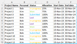
I want to take the data from sheet 1 and have the results in sheet 2.

I have a table that shows the Project name, status, allocation, start and end date, and the personal (Attached image)

I would like to have sheet 2 auto-populate a consolidated view. Sheet 2 Should show the Personal in one cell, The projects "In Progress" in another, the Allocation results in another and go red when over 100%, and then i am hoping for a chart that shows per month how much of the personals time will be taken up based on the start and end date of the projects in progress. (Attached is a mock view)

Any help would be great!

 

[Head Laker]

if you have not found an answer, Can you provide your workbook and i will have a look?

 

[Kay10]

Sheet 1 where all the information is kept.

Book1.xlsx
	E	F									O	P			S	T				X	Y	Z	AA	AB	AC
1	Overall Status	Project Name									Issue Date	Submitted Date			Issue Date 2	Submitted Date 2				Bid Lead	%	Proposal Lead	%2	Lead Estimator	%3
2
3
4
5
6
7
8
9
10
11
12
Sheet 1

Cells with Conditional Formatting
Cell	Condition		Cell Format	Stop If True
R2:U1048576	Cell	does not contain a blank value	text	NO
N2:Q497	Cell	does not contain a blank value	text	NO

Cells with Data Validation
Cell	Allow	Criteria
O2:P12	Date	between 01/01/2023 and 01/01/2030
S2:T12	Date	between 01/01/2023 and 01/01/2030
R1:T1	Any value

Sheet 2. Where i would like the view to be.

Book1.xlsx
	A	B	C	D	E	F	G	H	I	J	K	L	M	N	O	P	Q	R	S	T	U	V	W	X	Y	Z	AA	AB	AC	AD	AE	AF	AG	AH	AI	AJ	AK	AL	AM	AN	AO	AP	AQ	AR	AS	AT	AU	AV	AW	AX	AY	AZ	BA	BB	BC	BD	BE	BF
1	HIDE	January 1, 2024	1 - In Progress	January 22, 2024
2						2024
3						Jan					Feb				Mar				Apr					May				Jun				Jul					Aug				Sep					Oct				Nov				Dec
4	Project	Projects "In Progress"	Allocation %	Issue Date	Submit date	01-Jan	08-Jan	15-Jan	22-Jan	29-Jan	05-Feb	12-Feb	19-Feb	26-Feb	04-Mar	11-Mar	18-Mar	25-Mar	01-Apr	08-Apr	15-Apr	22-Apr	29-Apr	06-May	13-May	20-May	27-May	03-Jun	10-Jun	17-Jun	24-Jun	01-Jul	08-Jul	15-Jul	22-Jul	29-Jul	05-Aug	12-Aug	19-Aug	26-Aug	02-Sep	09-Sep	16-Sep	23-Sep	30-Sep	07-Oct	14-Oct	21-Oct	28-Oct	04-Nov	11-Nov	18-Nov	25-Nov	02-Dec	09-Dec	16-Dec	23-Dec	30-Dec
5	Personal 1
6
7
8
9
10
11
12
13
14
15		Total Overall Allocation	0%
Sheet 2

Cell Formulas
Range	Formula
D1	D1	=TODAY()
F3,K3,AT3	F3	=G4
O3,AK3,AO3,AX3	O3	=Q4
S3,X3,AB3,AF3,BB3	S3	=V4
G4:BF4	G4	=F4+7
F4	F4	=IF(MONTH(B1-WEEKDAY((B1),2)+1)<MONTH(B1),(B1-28-DAY(B1)+7)-WEEKDAY((B1-DAY(B1)+7),2)+1,(B1-DAY(B1)+7)-WEEKDAY((B1-DAY(B1)+7),2)+1)
F5	F5	=IFERROR(IFS((AND(#REF!>0,F$3>=#REF!,F$3<=$B5)),#REF!,(AND(F$3>=#REF!,F$3<=#REF!)),#REF!),"")
A5	A5	=Fields!A2
B5	B5	=IF(ROW()-ROW(B$5)+1<=SUM(--('Sheet 1'!$X$2:$X$300=A5)*('Sheet 1'!$E$2:$E$300=C1)), INDEX(FILTER('Sheet 1'!$F$2:$F$300, ('Sheet 1'!$X$2:$X$300=A5)*('Sheet 1'!$E$2:$E$300=C1)), ROW()-ROW(B$5)+1), "")
B6	B6	=IF(ROW()-ROW(B$5)+1<=SUM(--('Sheet 1'!$X$2:$X$300=A5)*('Sheet 1'!$E$2:$E$300=C1)), INDEX(FILTER('Sheet 1'!$F$2:$F$300, ('Sheet 1'!$X$2:$X$300=A5)*('Sheet 1'!$E$2:$E$300=C1)), ROW()-ROW(B$5)+1), "")
B7	B7	=IF(ROW()-ROW(B$5)+1<=SUM(--('Sheet 1'!$X$2:$X$300=A5)*('Sheet 1'!$E$2:$E$300=C1)), INDEX(FILTER('Sheet 1'!$F$2:$F$300, ('Sheet 1'!$X$2:$X$300=A5)*('Sheet 1'!$E$2:$E$300=C1)), ROW()-ROW(B$5)+1), "")
B8	B8	=IF(ROW()-ROW(B$5)+1<=SUM(--('Sheet 1'!$X$2:$X$300=A5)*('Sheet 1'!$E$2:$E$300=C1)), INDEX(FILTER('Sheet 1'!$F$2:$F$300, ('Sheet 1'!$X$2:$X$300=A5)*('Sheet 1'!$E$2:$E$300=C1)), ROW()-ROW(B$5)+1), "")
B9	B9	=IF(ROW()-ROW(B$5)+1<=SUM(--('Sheet 1'!$X$2:$X$300=A5)*('Sheet 1'!$E$2:$E$300=C1)), INDEX(FILTER('Sheet 1'!$F$2:$F$300, ('Sheet 1'!$X$2:$X$300=A5)*('Sheet 1'!$E$2:$E$300=C1)), ROW()-ROW(B$5)+1), "")
B10	B10	=IF(ROW()-ROW(B$5)+1<=SUM(--('Sheet 1'!$X$2:$X$300=A5)*('Sheet 1'!$E$2:$E$300=C1)), INDEX(FILTER('Sheet 1'!$F$2:$F$300, ('Sheet 1'!$X$2:$X$300=A5)*('Sheet 1'!$E$2:$E$300=C1)), ROW()-ROW(B$5)+1), "")
B11	B11	=IF(ROW()-ROW(B$5)+1<=SUM(--('Sheet 1'!$X$2:$X$300=A5)*('Sheet 1'!$E$2:$E$300=C1)), INDEX(FILTER('Sheet 1'!$F$2:$F$300, ('Sheet 1'!$X$2:$X$300=A5)*('Sheet 1'!$E$2:$E$300=C1)), ROW()-ROW(B$5)+1), "")
B12	B12	=IF(ROW()-ROW(B$5)+1<=SUM(--('Sheet 1'!$X$2:$X$300=A5)*('Sheet 1'!$E$2:$E$300=C1)), INDEX(FILTER('Sheet 1'!$F$2:$F$300, ('Sheet 1'!$X$2:$X$300=A5)*('Sheet 1'!$E$2:$E$300=C1)), ROW()-ROW(B$5)+1), "")
B13	B13	=IF(ROW()-ROW(B$5)+1<=SUM(--('Sheet 1'!$X$2:$X$300=A5)*('Sheet 1'!$E$2:$E$300=C1)), INDEX(FILTER('Sheet 1'!$F$2:$F$300, ('Sheet 1'!$X$2:$X$300=A5)*('Sheet 1'!$E$2:$E$300=C1)), ROW()-ROW(B$5)+1), "")
B14	B14	=IF(ROW()-ROW(B$5)+1<=SUM(--('Sheet 1'!$X$2:$X$300=A5)*('Sheet 1'!$E$2:$E$300=C1)), INDEX(FILTER('Sheet 1'!$F$2:$F$300, ('Sheet 1'!$X$2:$X$300=A5)*('Sheet 1'!$E$2:$E$300=C1)), ROW()-ROW(B$5)+1), "")
C5	C5	=IF(ROW()-ROW(B$5)+1<=SUM(--('Sheet 1'!$X$2:$X$300=A5)*('Sheet 1'!$E$2:$E$300=C1)), INDEX(FILTER('Sheet 1'!$Y$2:$Y$300, ('Sheet 1'!$X$2:$X$300=A5)*('Sheet 1'!$E$2:$E$300=C1)), ROW()-ROW(B$5)+1), "")
C6	C6	=IF(ROW()-ROW(B$5)+1<=SUM(--('Sheet 1'!$X$2:$X$300=A5)*('Sheet 1'!$E$2:$E$300=C1)), INDEX(FILTER('Sheet 1'!$Y$2:$Y$300, ('Sheet 1'!$X$2:$X$300=A5)*('Sheet 1'!$E$2:$E$300=C1)), ROW()-ROW(B$5)+1), "")
C7	C7	=IF(ROW()-ROW(B$5)+1<=SUM(--('Sheet 1'!$X$2:$X$300=A5)*('Sheet 1'!$E$2:$E$300=C1)), INDEX(FILTER('Sheet 1'!$Y$2:$Y$300, ('Sheet 1'!$X$2:$X$300=A5)*('Sheet 1'!$E$2:$E$300=C1)), ROW()-ROW(B$5)+1), "")
C8	C8	=IF(ROW()-ROW(B$5)+1<=SUM(--('Sheet 1'!$X$2:$X$300=A5)*('Sheet 1'!$E$2:$E$300=C1)), INDEX(FILTER('Sheet 1'!$Y$2:$Y$300, ('Sheet 1'!$X$2:$X$300=A5)*('Sheet 1'!$E$2:$E$300=C1)), ROW()-ROW(B$5)+1), "")
C9	C9	=IF(ROW()-ROW(B$5)+1<=SUM(--('Sheet 1'!$X$2:$X$300=A5)*('Sheet 1'!$E$2:$E$300=C1)), INDEX(FILTER('Sheet 1'!$Y$2:$Y$300, ('Sheet 1'!$X$2:$X$300=A5)*('Sheet 1'!$E$2:$E$300=C1)), ROW()-ROW(B$5)+1), "")
C10	C10	=IF(ROW()-ROW(B$5)+1<=SUM(--('Sheet 1'!$X$2:$X$300=A5)*('Sheet 1'!$E$2:$E$300=C1)), INDEX(FILTER('Sheet 1'!$Y$2:$Y$300, ('Sheet 1'!$X$2:$X$300=A5)*('Sheet 1'!$E$2:$E$300=C1)), ROW()-ROW(B$5)+1), "")
C11	C11	=IF(ROW()-ROW(B$5)+1<=SUM(--('Sheet 1'!$X$2:$X$300=A5)*('Sheet 1'!$E$2:$E$300=C1)), INDEX(FILTER('Sheet 1'!$Y$2:$Y$300, ('Sheet 1'!$X$2:$X$300=A5)*('Sheet 1'!$E$2:$E$300=C1)), ROW()-ROW(B$5)+1), "")
C12	C12	=IF(ROW()-ROW(B$5)+1<=SUM(--('Sheet 1'!$X$2:$X$300=A5)*('Sheet 1'!$E$2:$E$300=C1)), INDEX(FILTER('Sheet 1'!$Y$2:$Y$300, ('Sheet 1'!$X$2:$X$300=A5)*('Sheet 1'!$E$2:$E$300=C1)), ROW()-ROW(B$5)+1), "")
C13	C13	=IF(ROW()-ROW(B$5)+1<=SUM(--('Sheet 1'!$X$2:$X$300=A5)*('Sheet 1'!$E$2:$E$300=C1)), INDEX(FILTER('Sheet 1'!$Y$2:$Y$300, ('Sheet 1'!$X$2:$X$300=A5)*('Sheet 1'!$E$2:$E$300=C1)), ROW()-ROW(B$5)+1), "")
C14	C14	=IF(ROW()-ROW(B$5)+1<=SUM(--('Sheet 1'!$X$2:$X$300=A5)*('Sheet 1'!$E$2:$E$300=C1)), INDEX(FILTER('Sheet 1'!$Y$2:$Y$300, ('Sheet 1'!$X$2:$X$300=A5)*('Sheet 1'!$E$2:$E$300=C1)), ROW()-ROW(B$5)+1), "")
C15	C15	=SUM(C5:C14)

Cells with Conditional Formatting
Cell	Condition		Cell Format	Stop If True
F5	Expression	=AND(F$3>=#REF!,F$3<=#REF!)	text	NO
F6:DF15,G5:DF5	Expression	=AND(F$4>=#REF!-(WEEKDAY(#REF!,2)+1),F$4<=#REF!)	text	NO
F6:DF15,G5:DF5	Expression	=AND(F$4>=#REF!-(WEEKDAY(#REF!,2)+1),F$4<=#REF!)	text	NO
F6:DF15,G5:DF5	Expression	=AND(F$4>=#REF!-(WEEKDAY(#REF!,2)+1),F$4<=#REF!)	text	NO
F6:DF15,G5:DF5	Expression	=AND(F$4>=$B5-(WEEKDAY($B5,2)+1),F$4<=#REF!)	text	NO
F6:DF15,G5:DF5	Expression	=F$4=(TODAY()-WEEKDAY(TODAY(),2)+1)	text	NO