Countifs not working due to range ? maybe an array?

[mtleigh]

Hi and good afternoon,
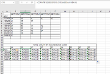
I am struggling to get a formula for countifs to work and i beleive this is due to my criteria ranges not being of the same size. Is there any work around to this?

i have put my example below but the actual data set is much larger but i have the same problem. the data set contains 15k rows and the worksheet is approx 25 columns in width.

so i have a table showing customer acc number and the service codes that may have been carried out throughout the year per customer per consignment hence why the same customer number may appear more than once. In the example above, the top table is my data set and the bottom of the 2 tables is a summary i am trying to get to work. I have tried named ranges instead of selecting the columns but this does not work either. If i try countif and count only the number of times the ACC appears it works, if i try countif to see how many times the service code appears, that also works, but i cannot get both to work in tandem using the countifs formula. I did read that both criteria ranges need to be of the same size. i did try then extending my acc criteria range to match the same number of columns but then it was only counting the first column of the service code range and not the other columns. Can anybody help?

 

[etaf]

try SUMPRODUCT()

excel forum-ETAF.xlsx
	A	B	C	D	E
1
2	1	1a	1b	1a
3	2	1b	1c	1a
4	1	1c		1a
5	2	1a	1b	1a
6	1	1b	1c	1a
7
8
9
10
11
12
13
14
15
16
17		1a	1b	1c
18	1	4	2	2
19	2	3	2	1
20
21
Sheet2

Cell Formulas
Range	Formula
B18:D19	B18	=SUMPRODUCT(($B$2:$D$6=B$17)*($A$2:$A$6=$A18))

 

[Fluff]

How about

=SUMPRODUCT(($B$3:$F$10=C$15)*($A$3:$A$10=$A17))

 

[mtleigh]

this works inmy example thankyou, however it does not work inmy dataset and i am unclear why. could it have anything to do with the service codes being a result of a formula and not a value on its own?

 

[etaf]

unlikely
but this quickly comes to mind

are the headings text - exactly the same as the text - no spaces
any issue where the numbers at the side are text in 1 table and not in another

Note: Images are difficult to see , and also requires that I input all the data myself, which means I may make an error, which is very time consuming, and from my point of view less likely to get a response, if a complicated spreadsheet. Plus we cannot see any of the formulas used.

Therefore -

A SMALL sample spreadsheet, around 10-20 rows, would help a lot here, with all sensitive data removed, and expected results mocked up and manually entered, with a few notes of explanation.

MrExcel has a tool called “XL2BB” that lets you post samples of your data and will allow us to copy/paste your sample data into our Excel spreadsheets, saving a lot of time.

XL2BB - Excel Range to BBCode

Excel 'mini-sheet' in messages - XL2BB Although experts prefer to read your description and question instead of working in your actual file to solve your problem, there are times that it is difficult to explain an issue without providing actual...

www.mrexcel.com

You can also test to see if it works ok, in the "Test Here" forum.

Test Here

Use this forum to test your signature, learn bbcode, smilies, XL2BB, etc. Threads in this forum are automatically deleted after no replies for seven (7) days

www.mrexcel.com

OR if you cannot get XL2BB to work, or have restrictions on your PC , then put the sample spreadsheet onto a share
I only tend to goto OneDrive, Dropbox or google docs , as I'm never certain of other random share sites and possible virus.
Please make sure you have a representative data sample and also that the data has been desensitised, remember this site is open to anyone with internet access to see - so any sensitive / personal data should be removed

 

[mtleigh]

in my dataset it comes back with 0 in every cell

 

[etaf]

do something like - where you expect a match

cell=cell
for both the account and the Service text

like F2 and G2 - in my example here

Book4
	A	B	C	D	E	F	G
1						TEST - acc	test Service
2	1	1a	1b	1a		TRUE	TRUE
3	2	1b	1c	1a
4	1	1c		1a
5	2	1a	1b	1a
6	1	1b	1c	1a
7
8
9
10
11
12
13
14
15
16
17		1a	1b	1c
18	1	4	2	2
19	2	3	2	1
20
Sheet1

Cell Formulas
Range	Formula
F2	F2	=A2=A18
G2	G2	=B2=B17
B18:D19	B18	=SUMPRODUCT(($B$2:$D$6=B$17)*($A$2:$A$6=$A18))

 

[mtleigh]

if they were in different formats then the countif formulas wouldnt work in the first place would they? as some of them are formula results they cannot be in text format and if i go to format cells on the summary sheet they are showing in 'General' format??

i think i have provided a link to Dropbox but not sure if it will work:

Special Services Check TMS by shipto.xlsm

Shared with Dropbox

www.dropbox.com

basically the sheet named 'By Shipto' in red needs summarisind as per by example earlier displayed. from the Data import sheet it is columns S:Z containing the codes which i need counting byt the ACC number which is in column B

 

[Fluff]

How about

=SUMPRODUCT((Report[[SC1]:[SC10]]=D$2)*(Report[[Shipto]:[Shipto]]=$A4))

 

[etaf]

i get it to work if i use the sheet name and range
=SUMPRODUCT(('Data Import'!$C$2:$L$20=D$2)*('Data Import'!$B$2:$B$20=$A4))

not sure what happens with the table references - when i include row 20 - it changes
to table reference
=SUMPRODUCT((Report[[SC1]:[SC10]]=D$2)*(Report[Shipto]=$A4))
But then returns zero

Not an expert at tables - and often have issues when referencing tables - i change to old reference sheet!range and usually get it to work

But no idea

will only be on dropbox for a couple of days

Special Services Check TMS by shipto - ETAF.xlsm

Shared with Dropbox

www.dropbox.com