Count (remove duplicate) in filter - Exel formula

[TH123]

Hi all,

Hope to get your support to solve this issue. I've searched in forum & there are many way to do but I still can't do with my data
Pls help to review this case & advise which Excel formula should be? (Not VBA or Pivot)

Below are What I want:
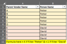
1. If I do filter at column B = Petter => formular at A11 will be shown = 4 (count parent vendor name with unique data)
2. If I do filter at column B = David => formular at A11 will be shown = 1 (count parent vendor name with unique data)

Thanks in advance.

 

[Fluff]

How about

=ROWS(UNIQUE(FILTER(A2:A10,B2:B10="Petter")))

 

[jdellasala]

It's a LOT easier to work with if the sample is posted using XL2BB or at least text. Also, you need someplace to chose what you're looking for.

It sounds like you're actually looking for a specific value in column A and need to specify what value you're looking for. Under that assumption:

Book1
	A	B
1	Parent Vendor Name	Person Name
2	A	Peter
3	B	Peter
4	B	Peter
5	C	Peter
6	D	Peter
7	E	David
8	E	David
9	E	David
10	E	David
11	1
12	Select Vendor:	E
Sheet1

Cell Formulas
Range	Formula
A11	A11	=IF(OR(B12="A",B12="B",B12="C",B12="D"),COUNTA(UNIQUE(FILTER(A2:A10,B2:B10="Peter"))),COUNTA(UNIQUE(FILTER(A2:A10,B2:B10="David"))))

Cells with Data Validation
Cell	Allow	Criteria
B12	List	=$A$2:$A$10

The formula could be extended using IFS instead of just IF, but it does get nasty!

I'm on the Insider Beta, so not sure if this has been released in the released version, but if you look at the formula for the Data Validation list, it includes the entire A2:A10 range, but presents a unique list - that is "B" is only listed once. It's a great enhancement of the Data Validation List, but it needs a Sort option.

 

[TH123]

How about

=ROWS(UNIQUE(FILTER(A2:A10,B2:B10="Petter")))

Hi Fluff,

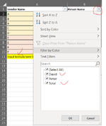
Thanks for your advice. It's much helpful if I create data validation separately however I'd like to input formula at row#11 as image => any other way to do if I select person name at column B then data will be linked automaticially at row#11?

I don't know how to upload mini-sheet => I've insert table below for your ref. Could you pls help?

Thank you.

Example: If I selected "Peter & Total" => result at row#11 should be 4.
If I selected "David & Total" => result at row#11 should be 1

Vendor Name (Column A)	Person Name (Column B)
A	Peter
B	Peter
B	Peter
C	Peter
D	Peter
E	David
E	David
E	David
E	David
Input formula here link with selection at column B	Total

 

[Fluff]

How about with a helper column

Fluff.xlsm
	A	B	C
1	Vendor Name	Person Name	Visible
2	A	Peter	1
3	B	Peter	1
4	B	Peter	1
5	C	Peter	1
6	D	Peter	1
7	E	David	1
8	E	David	1
9	E	David	1
10	E	David	1
11	5	Total
Sheet4

Cell Formulas
Range	Formula
C2:C10	C2	=SUBTOTAL(103,A2)
A11	A11	=ROWS(UNIQUE(FILTER(A2:A10,C2:C10=1)))

Fluff.xlsm
	A	B	C
1	Vendor Name	Person Name	Visible
2	A	Peter	1
3	B	Peter	1
4	B	Peter	1
5	C	Peter	1
6	D	Peter	1
11	4	Total
Sheet4

Cell Formulas
Range	Formula
C2:C6	C2	=SUBTOTAL(103,A2)
A11	A11	=ROWS(UNIQUE(FILTER(A2:A10,C2:C10=1)))

 

[TH123]

How about with a helper column

Fluff.xlsm
	A	B	C
1	Vendor Name	Person Name	Visible
2	A	Peter	1
3	B	Peter	1
4	B	Peter	1
5	C	Peter	1
6	D	Peter	1
7	E	David	1
8	E	David	1
9	E	David	1
10	E	David	1
11	5	Total
Sheet4

Cell Formulas
Range	Formula
C2:C10	C2	=SUBTOTAL(103,A2)
A11	A11	=ROWS(UNIQUE(FILTER(A2:A10,C2:C10=1)))

Fluff.xlsm
	A	B	C
1	Vendor Name	Person Name	Visible
2	A	Peter	1
3	B	Peter	1
4	B	Peter	1
5	C	Peter	1
6	D	Peter	1
11	4	Total
Sheet4

Cell Formulas
Range	Formula
C2:C6	C2	=SUBTOTAL(103,A2)
A11	A11	=ROWS(UNIQUE(FILTER(A2:A10,C2:C10=1)))

How intelligent you are! This is exactly what I want. Thanks for your help.

 

[Fluff]

You're welcome & thanks for the feedback.

 

[TH123]

Hi Fluff,

Sorry to disturb you again. I've another data & tried to apply same way but fail. What I need is in last column. Could you pls help to check my formula & adjust accordingly? Hope to get your reply soon. Thanks.

Book1
	A	B	C	D
1	Order#	Submit date	Formula (count how many time each order submit)	Needed
2	A	1-Dec	2	2
3	A	2-Dec	2	0
4	B	1-Dec	3	3
5	B	2-Dec	3	0
6	B	3-Dec	3	0
7	C	1-Dec	1	1
Sheet1

Cell Formulas
Range	Formula
C2:C7	C2	=ROWS(UNIQUE(FILTER($B$2:$B$7,$A$2:$A$7=A2)))

 

[TH123]

You're welcome & thanks for the feedback.

Hi Fluff,

Sorry, pls ignore my question in #8 above ( I can't delete it so pls just ignore).
My data as below. Logic is: Order#A, how many time submit late Yes & how many time submit late No as Needed data in last column. Could you pls support to give formula?
Thank you in advance.

Book1
	A	B	C	D	E
1	Order#	Submit date	Late submission?	Formula (count how many time each order submit)	Needed
2	A	1-Dec	No		1
3	A	2-Dec	Yes		1
4	B	1-Dec	No		1
5	B	2-Dec	Yes		2
6	C	1-Dec	No		1
7	A	1-Dec	No		0
8	B	3-Dec	Yes		0
Sheet1

 

[Fluff]

As this is a different question, it needs a new thread. Thanks