Copy and paste range in different sheet

achonikolov

New Member
Joined
May 28, 2012
Messages
17
Office Version
  1. 365
Platform
  1. Windows
Guys,

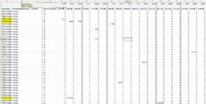
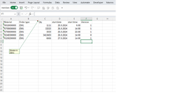
I need to copy some cells of different rows if i have value not equal to zero in cell.

If I have value not equal to zero need to copy sku code from the same row and then for quantity, start date, start time and version.

For example please see the attachments.
 

Attachments

  • Sheet1.png
    Sheet1.png
    190.6 KB · Views: 13
  • Sheet2.png
    Sheet2.png
    42.1 KB · Views: 12

Excel Facts

Show numbers in thousands?
Use a custom number format of #,##0,K. Each comma after the final 0 will divide the displayed number by another thousand
It is hard to work with a picture. It would be easier to help if you could use the XL2BB add-in (icon in the menu) to attach a screenshot (not a picture) of your sheet. Alternately, you could upload a copy of your file to a free site such as www.box.com or www.dropbox.com. Once you do that, mark it for 'Sharing' and you will be given a link to the file that you can post here. Explain in detail what you want to do referring to specific cells, rows, columns and sheets using a few examples from your data (de-sensitized if necessary).
 
Upvote 0
It would also be helpful to know which version of Excel you are on, as newer versions have some new functionality that may make this task easier.
I suggest that you update your Account details (or click your user name at the top right of the forum) so helpers always know what Excel version(s) & platform(s) you are using as the best solution often varies by version. (Don’t forget to scroll down & ‘Save’)
 
Upvote 0
It is hard to work with a picture. It would be easier to help if you could use the XL2BB add-in (icon in the menu) to attach a screenshot (not a picture) of your sheet. Alternately, you could upload a copy of your file to a free site such as www.box.com or www.dropbox.com. Once you do that, mark it for 'Sharing' and you will be given a link to the file that you can post here. Explain in detail what you want to do referring to specific cells, rows, columns and sheets using a few examples from your data (de-sensitized if necessary).


Link to download

1. If I have value different from 0 in area from "E" to "V" columns the macro needs to copy content from the same row in sheet1 to sheet2.
2. For example the first nonzero cell is "E6" from ""E" to "V"" area. At the row 6 the macro needs to copy first sku code from "A6" in sheet1 to "A2" in sheet2.
3. The column "B" in sheet2 always must be filled with "ZD01" .
4. Then the macro needs to copy "E6" from sheet and paste to "C2" in sheet2.
5. Copy "Е2" in sheet1 to "D2" in sheet2
6. Copy "E1" in sheet1 to "E2" in sheet2
7. Copy "C6" in sheet1 to "F2" in sheet2
And so on...until we finished with first date for each production line (L2, L5, L6, L7, L8)

The order must be:
1. starting date(26.09.)=>starting hour (06:00h) for L2
2. starting date(26.09.)=>starting hour (14:00h) for L2
3. starting date(26.09.)=>starting hour (22:00h) for L2
4. starting date(26.09.)=>starting hour (06:00h) for L5
5. starting date(26.09.)=>starting hour (14:00h) for L5
6. starting date(26.09.)=>starting hour (22:00h) for L5
7. starting date(26.09.)=>starting hour (06:00h) for L6
8. starting date(26.09.)=>starting hour (14:00h) for L6
9. starting date(26.09.)=>starting hour (22:00h) for L6
10. starting date(26.09.)=>starting hour (06:00h) for L7
11. starting date(26.09.)=>starting hour (14:00h) for L7
12. starting date(26.09.)=>starting hour (22:00h) for L7
13. starting date(26.09.)=>starting hour (06:00h) for L8
14. starting date(26.09.)=>starting hour (14:00h) for L8
15. starting date(26.09.)=>starting hour (22:00h) for L8

1. Next starting date(27.09.)=>starting hour (06:00h) for L2
2. Next starting date(27.09.)=>starting hour (14:00h) for L2
3. Next starting date(27.09.)=>starting hour (22:00h) for L2
4. Next starting date(27.09.)=>starting hour (06:00h) for L5
5. Next starting date(27.09.)=>starting hour (14:00h) for L5
6. Next starting date(27.09.)=>starting hour (22:00h) for L5
7. Next starting date(27.09.)=>starting hour (06:00h) for L6
8. Next starting date(27.09.)=>starting hour (14:00h) for L6
9. Next starting date(27.09.)=>starting hour (22:00h) for L6
10. Next starting date(27.09.)=>starting hour (06:00h) for L7
11. Next starting date(27.09.)=>starting hour (14:00h) for L7
12. Next starting date(27.09.)=>starting hour (22:00h) for L7
13. Next starting date(27.09.)=>starting hour (06:00h) for L8
14. Next starting date(27.09.)=>starting hour (14:00h) for L8
15. Next starting date(27.09.)=>starting hour (22:00h) for L8

And so on....until the end of the starting dates.


I hope that is enough but if you have any questions I will answer.
The link is available for 7 days.
Thank you in advance
 
Upvote 0

Try this, select the cells you want it to run on aor type the range in to the code.

VBA Code:
Sub MoveData()

Dim iRow As Integer
Dim iCol As Variant
Dim Addrow As Integer
Dim iSKU As Variant
Dim iQty As Variant
Dim iSDate As Variant
Dim iSTime As Variant
Dim iVersion As Variant

Addrow = Application.WorksheetFunction.CountA(Sheet2.Range("A:A")) + 1

For Each i In Range("E4:M9")  'Change for your data range

    If i.Value = 0 Then
    
    Else
    
    iRow = i.Row
    iCol = Split(Cells(1, Chr$(i.Column + 64)).Address, "$")(1)
    
    iQty = i.Value
    iSKU = Range("A" & iRow).Value
    iSDate = Range(iCol & "3").Value
    iSTime = Range(iCol & "1").Value
    iVersion = Range("C" & iRow).Value
    
    With Sheet2
    .Range("A" & Addrow) = iSKU
    .Range("B" & Addrow) = "ZD01"
    .Range("C" & Addrow) = iQty
    .Range("D" & Addrow) = iSDate
    .Range("E" & Addrow) = iSTime
    .Range("F" & Addrow) = iVersion
    End With
    Addrow = Addrow + 1
    End If

Next i

End Sub

My crude mockup of your data and the results....
1727946693938.png


1727946715793.png
 
Upvote 0

Try this, select the cells you want it to run on aor type the range in to the code.

VBA Code:
Sub MoveData()

Dim iRow As Integer
Dim iCol As Variant
Dim Addrow As Integer
Dim iSKU As Variant
Dim iQty As Variant
Dim iSDate As Variant
Dim iSTime As Variant
Dim iVersion As Variant

Addrow = Application.WorksheetFunction.CountA(Sheet2.Range("A:A")) + 1

For Each i In Range("E4:M9")  'Change for your data range

    If i.Value = 0 Then
   
    Else
   
    iRow = i.Row
    iCol = Split(Cells(1, Chr$(i.Column + 64)).Address, "$")(1)
   
    iQty = i.Value
    iSKU = Range("A" & iRow).Value
    iSDate = Range(iCol & "3").Value
    iSTime = Range(iCol & "1").Value
    iVersion = Range("C" & iRow).Value
   
    With Sheet2
    .Range("A" & Addrow) = iSKU
    .Range("B" & Addrow) = "ZD01"
    .Range("C" & Addrow) = iQty
    .Range("D" & Addrow) = iSDate
    .Range("E" & Addrow) = iSTime
    .Range("F" & Addrow) = iVersion
    End With
    Addrow = Addrow + 1
    End If

Next i

End Sub

My crude mockup of your data and the results....
View attachment 117637

View attachment 117638
Hi sxhall,

Thank you so much and looks great!

But the order in sheet2 must be:
1. starting date(26.09.)=>starting hour (06:00h) for L2
2. starting date(26.09.)=>starting hour (14:00h) for L2
3. starting date(26.09.)=>starting hour (22:00h) for L2
4. starting date(26.09.)=>starting hour (06:00h) for L5
5. starting date(26.09.)=>starting hour (14:00h) for L5
6. starting date(26.09.)=>starting hour (22:00h) for L5
7. starting date(26.09.)=>starting hour (06:00h) for L6
8. starting date(26.09.)=>starting hour (14:00h) for L6
9. starting date(26.09.)=>starting hour (22:00h) for L6
10. starting date(26.09.)=>starting hour (06:00h) for L7
11. starting date(26.09.)=>starting hour (14:00h) for L7
12. starting date(26.09.)=>starting hour (22:00h) for L7
13. starting date(26.09.)=>starting hour (06:00h) for L8
14. starting date(26.09.)=>starting hour (14:00h) for L8
15. starting date(26.09.)=>starting hour (22:00h) for L8

1. Next starting date(27.09.)=>starting hour (06:00h) for L2
2. Next starting date(27.09.)=>starting hour (14:00h) for L2
3. Next starting date(27.09.)=>starting hour (22:00h) for L2
4. Next starting date(27.09.)=>starting hour (06:00h) for L5
5. Next starting date(27.09.)=>starting hour (14:00h) for L5
6. Next starting date(27.09.)=>starting hour (22:00h) for L5
7. Next starting date(27.09.)=>starting hour (06:00h) for L6
8. Next starting date(27.09.)=>starting hour (14:00h) for L6
9. Next starting date(27.09.)=>starting hour (22:00h) for L6
10. Next starting date(27.09.)=>starting hour (06:00h) for L7
11. Next starting date(27.09.)=>starting hour (14:00h) for L7
12. Next starting date(27.09.)=>starting hour (22:00h) for L7
13. Next starting date(27.09.)=>starting hour (06:00h) for L8
14. Next starting date(27.09.)=>starting hour (14:00h) for L8
15. Next starting date(27.09.)=>starting hour (22:00h) for L8

And so on....until the end of the starting dates.

MaterialOrder typeQtystart datestart timeVersionProd line
70060000000​
ZD01
11​
26.9.2024​
6:00​
0​
L2
70060000000​
ZD01
23​
26.9.2024​
14:00​
0​
L5
70060000000​
ZD01
22​
26.9.2024​
22:00​
0​
L7
70150100000​
ZD01
25​
26.9.2024​
14:00​
1​
L8
70150200000​
ZD01
12​
27.9.2024​
14:00​
1​
L2
70510000000​
ZD01
13​
27.9.2024​
6:00​
1​
L2
70510000000​
ZD01
36​
27.9.2024​
22:00​
1​
L5
70510200000​
ZD01
166​
27.9.2024​
14:00​
1​
L6
70510200000​
ZD01
21​
27.9.2024​
22:00​
1​
L7
70700000000​
ZD01
31​
27.9.2024​
14:00​
1​
L8

Wait...sorting by "starting date", then by "starting time" and "Prod line" will be perfect.
 
Upvote 0
Try:
VBA Code:
Sub CopyData()
    Application.ScreenUpdating = False
    Dim v As Variant, r As Long, c As Long, srcWS As Worksheet, desWS As Worksheet, lCol As Long
    Set srcWS = Sheets("Sheet1")
    Set desWS = Sheets("Sheet2")
    lCol = srcWS.Cells(1, srcWS.Columns.Count).End(xlToLeft).Column
    v = srcWS.Range("A1", srcWS.Range("A" & Rows.Count).End(xlUp)).Resize(, lCol).Value
    For c = 5 To UBound(v, 2)
        For r = 4 To UBound(v)
            If v(r, c) <> 0 Then
                With desWS
                    .Cells(.Rows.Count, "A").End(xlUp).Offset(1).Resize(, 6).Value = Array(v(r, 1), "ZD01", v(r, 5), v(3, c), Format(v(1, c), "h:mm"), v(r, 3))
                End With
            End If
        Next r
    Next c
    Application.ScreenUpdating = True
End Sub
 
Upvote 0
Sorry. Please try this version:
VBA Code:
Sub CopyData()
    Application.ScreenUpdating = False
    Dim v As Variant, r As Long, c As Long, srcWS As Worksheet, desWS As Worksheet, lCol As Long
    Set srcWS = Sheets("Sheet1")
    Set desWS = Sheets("Sheet2")
    lCol = srcWS.Cells(1, srcWS.Columns.Count).End(xlToLeft).Column
    v = srcWS.Range("A1", srcWS.Range("A" & Rows.Count).End(xlUp)).Resize(, lCol).Value
    For r = 4 To UBound(v)
        For c = 5 To UBound(v, 2)
            If v(r, c) > 0 Then
                With desWS
                    .Cells(.Rows.Count, "A").End(xlUp).Offset(1).Resize(, 6).Value = Array(v(r, 1), "ZD01", v(r, c), v(3, c), Format(v(1, c), "h:mm"), v(r, 3))
                End With
            End If
        Next c
    Next r
    Application.ScreenUpdating = True
End Sub
 
Upvote 0
Solution
OK have captured the Prod Line now as well and included a sort at the end...

VBA Code:
Sub MoveData()

Dim iRow As Integer
Dim iCol As Variant
Dim Addrow As Integer
Dim iSKU As Variant
Dim iQty As Variant
Dim iSDate As Variant
Dim iSTime As Variant
Dim iProd As Variant
Dim iVersion As Variant

Addrow = Application.WorksheetFunction.CountA(Sheet2.Range("A:A")) + 1

For Each i In Range("E4:M9")

    If i.Value = 0 Then
    
    Else
    
    iRow = i.Row
    iCol = Split(Cells(1, Chr$(i.Column + 64)).Address, "$")(1)
    
    iQty = i.Value
    iSKU = Range("A" & iRow).Value
    iSDate = Range(iCol & "3").Value
    iSTime = Range(iCol & "1").Value
    iVersion = Range("C" & iRow).Value
    iProd = Range("D" & iRow).Value
    
    With Sheet2
    .Range("A" & Addrow) = iSKU
    .Range("B" & Addrow) = "ZD01"
    .Range("C" & Addrow) = iQty
    .Range("D" & Addrow) = iSDate
    .Range("E" & Addrow) = iSTime
    .Range("F" & Addrow) = iVersion
    .Range("G" & Addrow) = iProd
    End With
    Addrow = Addrow + 1
    End If

Next i

With ActiveWorkbook.Worksheets("Sheet2")
    .Sort.SortFields.Clear
    .Sort.SortFields.Add2 Key:=Range("D2:D" & Addrow) _
        , SortOn:=xlSortOnValues, Order:=xlAscending, DataOption:=xlSortNormal
    .Sort.SortFields.Add2 Key:=Range("E2:E" & Addrow) _
        , SortOn:=xlSortOnValues, Order:=xlAscending, DataOption:=xlSortNormal
    .Sort.SortFields.Add2 Key:=Range("G2:G" & Addrow) _
        , SortOn:=xlSortOnValues, Order:=xlAscending, DataOption:=xlSortNormal
End With
    With ActiveWorkbook.Worksheets("Sheet2").Sort
        .SetRange Range("A1:G" & Addrow)
        .Header = xlYes
        .MatchCase = False
        .Orientation = xlTopToBottom
        .SortMethod = xlPinYin
        .Apply
    End With

End Sub

My result...

1727965605283.png
 
Upvote 0
Thank you guys!!!

You save me hours of copying and pasting.

I appreciate your help.
 
Upvote 0

Forum statistics

Threads
1,223,908
Messages
6,175,306
Members
452,633
Latest member
DougMo

We've detected that you are using an adblocker.

We have a great community of people providing Excel help here, but the hosting costs are enormous. You can help keep this site running by allowing ads on MrExcel.com.
Allow Ads at MrExcel

Which adblocker are you using?

Disable AdBlock

Follow these easy steps to disable AdBlock

1)Click on the icon in the browser’s toolbar.
2)Click on the icon in the browser’s toolbar.
2)Click on the "Pause on this site" option.
Go back

Disable AdBlock Plus

Follow these easy steps to disable AdBlock Plus

1)Click on the icon in the browser’s toolbar.
2)Click on the toggle to disable it for "mrexcel.com".
Go back

Disable uBlock Origin

Follow these easy steps to disable uBlock Origin

1)Click on the icon in the browser’s toolbar.
2)Click on the "Power" button.
3)Click on the "Refresh" button.
Go back

Disable uBlock

Follow these easy steps to disable uBlock

1)Click on the icon in the browser’s toolbar.
2)Click on the "Power" button.
3)Click on the "Refresh" button.
Go back
Back
Top