Convert Formula from .xlsx Version to .xls

pineapple61

New Member
Joined
Jan 31, 2023
Messages
7
Office Version
  1. 365
  2. 2021
  3. 2016
Platform
  1. Windows
  2. MacOS
Hi everyone, someone helped me create a formula to filter an excel sheet (the thread post can be found here: Filtering One Condition to Multiple Columns on a Drop Down List). However, since I created this formula on the Office 365, 2021 version (.xlsx), when I open the file in the Office 2016 version (.xls) the formulas are no longer valid. I tried converting the file from .xlsx to .xls but it did not work. Could anyone help me with this?


Book1.xlsx
ABCDEFGHI
1NameFirst JobSecond JobThird JobDoctor
2JohnDoctorPoliceMechanicNameFirst JobSecond JobThird Job
3MarcusFiremanSalesmanWaiterJohnDoctorPoliceMechanic
4KyleDoctorEngineerFiremanKyleDoctorEngineerFireman
5AlexaEngineerDoctorDoctorBritneyDoctorMechanicWaitress
6BritneyDoctorMechanicWaitressAlexaEngineerDoctorDoctor
7FergusonPoliceFiremanEngineer
Test
Cell Formulas
RangeFormula
F3:I6F3=UNIQUE(VSTACK(FILTER($A$2:$D$7,$B$2:$B$7=G1,""),FILTER($A$2:$D$7,$C$2:$C$7=G1,""),FILTER($A$2:$D$7,$D$2:$D$7=G1,"")))
Dynamic array formulas.
Cells with Data Validation
CellAllowCriteria
F1:G1ListDoctor, Fireman, Engineer, Police, Salesman, Mechanic, Waiter, Waitress
 

Excel Facts

Add Bullets to Range
Select range. Press Ctrl+1. On Number tab, choose Custom. Type Alt+7 then space then @ sign (using 7 on numeric keypad)
It is not xls vs xlsx. The functions VSTACK, FILTER, and UNIQUE are not available in Excel 2016. You'll have to build the equation differently.
 
Upvote 0
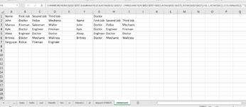
Try this ctrl shift enter if you're not on 365

Excel Formula:
=IFERROR(INDEX($A$2:$D$7,AGGREGATE(15,6,ROW($A$2:$A$7)/--(FREQUENCY(IF($B$2:$D$7=$G$1,ROW($A$2:$A$7)),ROW($A$2:$A$7))>0)-1,ROW($A1)),COLUMN(A$1)),"")
 

Attachments

  • 1675414822040.png
    1675414822040.png
    33.5 KB · Views: 7
Upvote 0
Another option
Fluff.xlsm
ABCDEFGHI
1NameFirst JobSecond JobThird JobDoctor
2JohnDoctorPoliceMechanicNameFirst JobSecond JobThird Job
3MarcusFiremanSalesmanWaiterJohnDoctorPoliceMechanic
4KyleDoctorEngineerFiremanKyleDoctorEngineerFireman
5AlexaEngineerDoctorDoctorAlexaEngineerDoctorDoctor
6BritneyDoctorMechanicWaitressBritneyDoctorMechanicWaitress
7FergusonPoliceFiremanEngineer    
8
Main
Cell Formulas
RangeFormula
F3:I7F3=IFERROR(INDEX(A:A,AGGREGATE(15,6,ROW($A$2:$A$7)/($B$2:$D$7=$G$1)/(ISNA(MATCH($A$2:$A$7,$F$2:$F2,0))),1)),"")
 
Upvote 0
Try this ctrl shift enter if you're not on 365

Excel Formula:
=IFERROR(INDEX($A$2:$D$7,AGGREGATE(15,6,ROW($A$2:$A$7)/--(FREQUENCY(IF($B$2:$D$7=$G$1,ROW($A$2:$A$7)),ROW($A$2:$A$7))>0)-1,ROW($A1)),COLUMN(A$1)),"")
It worked! This made me so happy, you are a lifesaver!!!!!!!!!
 
Upvote 0
Another option
Fluff.xlsm
ABCDEFGHI
1NameFirst JobSecond JobThird JobDoctor
2JohnDoctorPoliceMechanicNameFirst JobSecond JobThird Job
3MarcusFiremanSalesmanWaiterJohnDoctorPoliceMechanic
4KyleDoctorEngineerFiremanKyleDoctorEngineerFireman
5AlexaEngineerDoctorDoctorAlexaEngineerDoctorDoctor
6BritneyDoctorMechanicWaitressBritneyDoctorMechanicWaitress
7FergusonPoliceFiremanEngineer    
8
Main
Cell Formulas
RangeFormula
F3:I7F3=IFERROR(INDEX(A:A,AGGREGATE(15,6,ROW($A$2:$A$7)/($B$2:$D$7=$G$1)/(ISNA(MATCH($A$2:$A$7,$F$2:$F2,0))),1)),"")
This formula also worked! Thank you so so much, you guys are the best!
 
Upvote 0
Glad we could help & thanks for the feedback.
 
Upvote 0

Forum statistics

Threads
1,223,236
Messages
6,170,917
Members
452,366
Latest member
TePunaBloke

We've detected that you are using an adblocker.

We have a great community of people providing Excel help here, but the hosting costs are enormous. You can help keep this site running by allowing ads on MrExcel.com.
Allow Ads at MrExcel

Which adblocker are you using?

Disable AdBlock

Follow these easy steps to disable AdBlock

1)Click on the icon in the browser’s toolbar.
2)Click on the icon in the browser’s toolbar.
2)Click on the "Pause on this site" option.
Go back

Disable AdBlock Plus

Follow these easy steps to disable AdBlock Plus

1)Click on the icon in the browser’s toolbar.
2)Click on the toggle to disable it for "mrexcel.com".
Go back

Disable uBlock Origin

Follow these easy steps to disable uBlock Origin

1)Click on the icon in the browser’s toolbar.
2)Click on the "Power" button.
3)Click on the "Refresh" button.
Go back

Disable uBlock

Follow these easy steps to disable uBlock

1)Click on the icon in the browser’s toolbar.
2)Click on the "Power" button.
3)Click on the "Refresh" button.
Go back
Back
Top