Conditional SUMPRODUCT Formula

[brandonej]

Hello all. I need a formula that sums an array of values based on certain criteria.

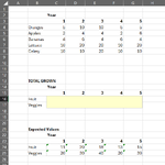
The attached image is a simplified dataset for reference (the actual dataset is significantly larger).

Logic (for fruit): IF B4:B8 (item category) = oranges, OR apples, OR bananas, AND IF C15 (the year) matches C3:G3, return the SUMPRODUCT of the entire array C4:G8.

The logic is similar for veggies.

I tried to use IF AND OR SUMPRODUCT with no success.

Here is the formula I tried to use for fruit: =IF(AND(OR(B4:B8="Oranges","Apples","Bananas"),C15=$C$3:$G$3),SUMPRODUCT($C$4:$G$8))

 

[Eric W]

How about:

Book1
	A	B	C	D	E	F	G	H	I	J
1
2			Year						Fruit	Veggies
3			1	2	3	4	5		Oranges	Lettuce
4		Oranges	5	10	10	5	5		Apples	Celery
5		Apples	2	4	4	2	6		Bananas
6		Bananas	4	6	4	6	4
7		Lettuce	10	20	20	10	20
8		Celery	10	10	20	10	10
9
10
11
12
13		TOTAL GROWN
14			Year
15			1	2	3	4	5
16		Fruit	11	20	18	13	15
17		Veggies	20	30	40	20	30
18
Sheet9

Cell Formulas
Range	Formula
C16:G17	C16	=SUM(C$4:C$8*COUNTIF(INDEX($I$3:$J$10,0,MATCH($B16,$I$2:$J$2,0)),$B$4:$B$8))

I made a table for the fruits and veggies to make it easy to update.

 

[brandonej]

How about:

Book1
	A	B	C	D	E	F	G	H	I	J
1
2			Year						Fruit	Veggies
3			1	2	3	4	5		Oranges	Lettuce
4		Oranges	5	10	10	5	5		Apples	Celery
5		Apples	2	4	4	2	6		Bananas
6		Bananas	4	6	4	6	4
7		Lettuce	10	20	20	10	20
8		Celery	10	10	20	10	10
9
10
11
12
13		TOTAL GROWN
14			Year
15			1	2	3	4	5
16		Fruit	11	20	18	13	15
17		Veggies	20	30	40	20	30
18
Sheet9

Cell Formulas
Range	Formula
C16:G17	C16	=SUM(C$4:C$8*COUNTIF(INDEX($I$3:$J$10,0,MATCH($B16,$I$2:$J$2,0)),$B$4:$B$8))

I made a table for the fruits and veggies to make it easy to update.

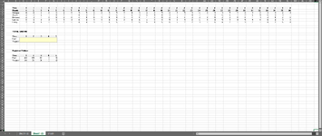
Thank you for your help. However, that solution might not work for the larger dataset I referenced in my post.

I should've added that I need a solution that works even if the fruits and veggies data is more granular (e.g., monthly).

(See snapshot for reference.)

 

[Eric W]

That's a risk if you simplify your data too much, the results might not be valid to your entire data. In this case, it's not too hard to adapt:

Book1
	A	B	C	D	E	F	G	H	I	J	K	L	M
1
2
3		Year	1	1	1	1	1	2	2	2	2	2
4		Month	1	2	3	4	5	1	2	3	4	5
5		Oranges	5	10	10	5	5	14	10	20	8	5
6		Apples	2	4	4	2	6	2	3	14	14	14
7		Bananas	4	6	4	6	4	2	16	7	17	3
8		Lettuce	10	20	20	10	20	9	12	11	8	9
9		Celery	10	10	20	10	10	5	16	20	13	17
10
11
12
13		TOTAL GROWN
14			Year
15			1	2	3	4	5
16		Fruit	77	149	0	0	0
17		Veggies	140	120	0	0	0
18
19
20		Fruit	Veggies
21		Oranges	Lettuce
22		Apples	Celery
23		Bananas
24
Sheet9

Cell Formulas
Range	Formula
C16:G17	C16	=SUM($C$5:$L$9*COUNTIF(INDEX($B$21:$C$28,0,MATCH($B16,$B$20:$C$20,0)),$B$5:$B$9)*($C$3:$L$3=C$15))

 

[brandonej]

That works. Thank you!