Conditional Formula

[santoshloka]

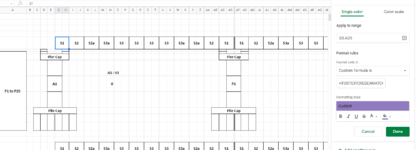
Looking for formula in google sheets

=IF(ISTEXT(REGEXMATCH(G5:AD5, VLOOKUP(E10&"-"&AD10,N9:O9,2,TRUE))), 1, 0)-->I want formula (Color Not Visible)

=IF(regexmatch( "G5:AD5", "S1"), 1, 0)-->Option working in conditional Formatting(Color Visible)

Please find the image
when N9:O9=S1 IS TRUE then match that text in G5 to AD5 Then give a color

 

[Peter_SSs]

Looking for formula in google sheets

Then please ask in the appropriate forum (I have moved it for you this time)

 

[santoshloka]

Hi,

Thanks for the update

This formula is not working in excel also

 

[Peter_SSs]

This formula is not working in excel also

It would not be expected to work in Excel since Excel does not have a REGEXMATCH function.

 

[santoshloka]

I'm trying to make a condition if the name S1 or S2 on O9..I want the color in G5:AD5

if possible can you please help me with formula

 

[Peter_SSs]

I'm trying to make a condition if the name S1 or S2 on O9..I want the color in G5:AD5

I have no idea what that means.