Conditional Formatting

[GetGemmafied]

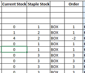
Help. I am trying to create a rule where a cell changes colour based on the values of other cells.
I have created a Stocktake and order form. I am trying to have the cell in the "ORDER" column change colour when the cell in the "Stocktake" column is less then the cell in the "Staple" Column. Does that make sense?
I appreciate any and all help. Thank you

 

[Peter_SSs]

Welcome to the MrExcel board!

Something like this?

24 08 23.xlsm
	D	E	F	G
7	0	1		1
8	1	2		1
9	4	2		-2
10	0	1		1
CF

Cells with Conditional Formatting
Cell	Condition		Cell Format	Stop If True
G7:G10	Expression	=D7<E7	text	NO

BTW, I suggest that you investigate XL2BB for providing sample data to make it easier for helpers by not having to manually type out sample data to test with. If you have trouble with XL2BB review the "XL2BB Icons greyed out" link in the 'Known XL2BB issues' section near the top of theXL2BB Instructions page linked above.

 

[GetGemmafied]

Welcome to the MrExcel board!

Something like this?

24 08 23.xlsm
	D	E	F	G
7	0	1		1
8	1	2		1
9	4	2		-2
10	0	1		1
CF

Cells with Conditional Formatting
Cell	Condition		Cell Format	Stop If True
G7:G10	Expression	=D7<E7	text	NO

BTW, I suggest that you investigate XL2BB for providing sample data to make it easier for helpers by not having to manually type out sample data to test with. If you have trouble with XL2BB review the "XL2BB Icons greyed out" link in the 'Known XL2BB issues' section near the top of theXL2BB Instructions page linked above.

Thank you Peter, much appreciated. Where do I put this formula?

 

[Peter_SSs]

Where do I put this formula?

For the layout in my sample

Select from G7:G10 and then
Home ribbon tab -> Conditional Formatting -> New rule ... -> Use a formula to determine which cells to format -> Format values where this formula is true: =D7<E7 -> Format... -> Set whatever formatting you want -> OK -> OK

 

[GetGemmafied]

For the layout in my sample

Select from G7:G10 and then
Home ribbon tab -> Conditional Formatting -> New rule ... -> Use a formula to determine which cells to format -> Format values where this formula is true: =D7<E7 -> Format... -> Set whatever formatting you want -> OK -> OK

Awesome, thank you so much. Very much appreciated

 

[Peter_SSs]

You're welcome. Thanks for the follow-up.