Conditional Formatting Will NOT stay true

[WhatTheF]

I'm at the end of my rope on this one. I've looked, and I can't find anyone else having this issue.

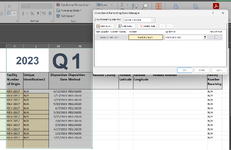
I've got 19 Columns, A:S. At the top, there are a few merged cells that get in the way of just Conditional Formatting the entire columns. There's nothing I can do about that. My problem is, the Conditional Formatting only works on most of the cells in the range, and then, it changes every time I click "OK" to create a New Rule.

If the cells contain anything at all, I need to highlight all of the cells in from A3:Dwherever_they_ stop, in Color1, E3:Fwherever_they_ stop in Color2, G3:Jwherever_they_ stop in Color3, K3:Lwherever_they_ stop in Color4, M3:Nwherever_they_ stop in Color2, O3:Rwherever_they_ stop in Color3, and S3:Swherever_they_ stop in Color5.

There are not Rules previously applied to the workbook, anywhere, and there are no strange formats applied anywhere. The information is being Copy/Paste_Values from another workbook through a Macro. I can't paint in the formula manually, as this needs to be part of the same macro, so others can't (HA! Right!) screw it up later. The only formatting is Row/Column sizes. Every time I input my formula for the Conditional Formatting, [Conditional Formatting>New Rule>=A1<>"" > Format>Chose_Colors/Border>OK>OK], It changes from A1 to A3 or A5. When I go back in and change the range for it to be applied to from $A$1 to $A$3:$A$1000, it changes the Formula value to random places on the sheet...

I'm so frustrated I want to bite something!

Can someone please help me get this figured out so I don't start considering fire as an option!

 

[etaf]

sometimesi get "" around the formula
and if i change ranges - I can get ti save as A1033334556 - some number not sure which

If you select the range as A3:A1000 , then the formula needs to start in row 3
so =A3<>""

will highlight every thing in that column that is not blank

where are the merged cells ?

 

[kvsrinivasamurthy]

Select A1:A1000 with A1 as active cell.
Now enter formula for CF
A1<>""

 

[WhatTheF]

I'm not sure if this will show the CF code or not, but these are the kinds of issues I keep running into:

In the attached image, you can see at the bottom there is no information in the four highlighted squares, and at the top right, there IS information in a square that is not highlighted. This exact same code [Cell K1 selected > CF > =K1<>"" > Format > Color > Border > OK > OK > Applies To: =$K$3:$L$1000 (when I type ":", it autofills with "$K$3$K$3:$L$1000" and I have to delete back to $K$3 and type ":" again, along with the range it should apply) > Apply > OK] worked perfectly when I used it a few minutes ago. It also appears to have worked perfectly in Columns A:J. However, for whatever reason, it's not working this time.

Also, when I'm recording my Macro, none of the CF range changes are recorded. It just applies it to $A$3, or whatever cell is selected when I first write it.

Here's my Mini Sheet that will, hopefully show what's going on:

TPW Quarterly Report Generator.xlsx
	H	I	J	K	L	M
1	PERM-42071			2023		Q
2	Collection Latitude	Collection Longitude	Collection Address	Facility Number of Origin	Unique Identification2	Disposition Date
3	UNKNOWN	UNKNOWN	UNKNOWN	REH-2017	N/A	6/12/2023
4	UNKNOWN	UNKNOWN	UNKNOWN	REH-2017	N/A	2/17/2023
5	UNKNOWN	UNKNOWN	UNKNOWN	REH-2017	N/A	3/29/2023
6	UNKNOWN	UNKNOWN	UNKNOWN	REH-2017	N/A	5/20/2023
7	UNKNOWN	UNKNOWN	UNKNOWN	REH-2017	N/A	6/7/2023
8	UNKNOWN	UNKNOWN	UNKNOWN	REH-2017	N/A	5/30/2023
9	UNKNOWN	UNKNOWN	UNKNOWN	REH-2017	N/A	1/21/2023
10	UNKNOWN	UNKNOWN	UNKNOWN	REH-2017	N/A	2/6/2023
11	UNKNOWN	UNKNOWN	UNKNOWN	REH-2017	N/A	2/9/2023
12	UNKNOWN	UNKNOWN	UNKNOWN	REH-2017	N/A	4/17/2023
13	UNKNOWN	UNKNOWN	UNKNOWN	REH-2017	N/A	6/6/2023
14	UNKNOWN	UNKNOWN	UNKNOWN	REH-2017	N/A	4/21/2023
15
16
17
Sheet1

Cells with Conditional Formatting
Cell	Condition		Cell Format	Stop If True
K3:L1000	Expression	=K1<>""	text	NO
G3:J1000	Expression	=G3<>""	text	NO

 

[Peter_SSs]

Everything that you describe and show in your mini sheets/pictures indicates that you applied the CF formula =K1<>"" when you had K3:L1000 selected.
If you remove all CF from columns K:L, select K3:L1000 and apply the CF rule =K3<>"" it should be right.

BTW, this is what @etaf already indicated in post #2 (though in relation to a different column)

If you select the range as A3:A1000 , then the formula needs to start in row 3
so =A3<>""

 

[WhatTheF]

Everything that you describe and show in your mini sheets/pictures indicates that you applied the CF formula =K1<>"" when you had K3:L1000 selected.
If you remove all CF from columns K:L, select K3:L1000 and apply the CF rule =K3<>"" it should be right.

That's the problem I'm having. When I Enter "=K3<>""" and go through the rest of the process, as soon as I OK out after Appling it, it changes the formula. It's always by two rows. Sometimes it changes it to K1, others it's K5. (Or whatever Column/Row I'm working with. It's not limited to K1/3/5.) I'm trying to figure out if there's some weird setting I'm missing, here, or if there's some kind of glitch in my copy of Excel.

 

[Peter_SSs]

You have not confirmed specifically that you have had the correct selection made when applying the CF & I still believe that is causing your problem.

Did you follow these steps exactly?

If you remove all CF from columns K:L, select K3:L1000 and apply the CF rule =K3<>""

Note that the selection before applying the rule is not the whole columns. Your active cell must be K3, not K1 from selecting the whole column. This is what your sheet should look like before you go into Conditional formatting to apply the rule. Note the active cell (unshaded) is K3

 

[WhatTheF]

Note that the selection before applying the rule is not the whole columns. Your active cell must be K3, not K1 from selecting the whole column. This is what your sheet should look like before you go into Conditional formatting to apply the rule. Note the active cell (unshaded) is K3

I am creating the CF while the selected, active cell is, in this case, K3. As I move along, the Column changes, but the selected cell is the upper-most left cell, always on Row 3 in this case. I am not, however, selecting 1,994/3,888 cells before I open the CF dialog. I'm selecting/activating the first cell, in this case, K3, entering the formula, "K3<>""", choosing the format color and border, OK, OK, then changing the "Applies To" range next to the formula in the Manage Rules dialog box.

I'm starting to think it might be time to re-install Excel... It will, literally, work perfectly fine for two or three runs of the formulas on the page, then change, too... Something is not working correctly. Normally, I'd agree that's it's the loose screw on the keyboard...! But I've been over this too many times, at this point!

 

[Peter_SSs]

I'm selecting/activating the first cell, in this case, K3, entering the formula, "K3<>""", choosing the format color and border, OK, OK, then changing the "Applies To" range next to the formula in the Manage Rules dialog box.

Ok, thanks for confirming. In that case the things that come to mind are ..

• Some vba code in the workbook is messing with the CF
• The workbook is corrupt. It would be best to try to determine if it is the workbook rather than Excel causing the problem. So before reinstalling Excel I would consider copying the data (not the CF) to a band new workbook, apply the CF in that new workbook and work with that for a while to see if the same thing happens. Do you have any other workbooks with CF? If so, are they misbehaving?

 

[WhatTheF]

Ok, thanks for confirming. In that case the things that come to mind are ..

• Some vba code in the workbook is messing with the CF
• The workbook is corrupt. It would be best to try to determine if it is the workbook rather than Excel causing the problem. So before reinstalling Excel I would consider copying the data (not the CF) to a band new workbook, apply the CF in that new workbook and work with that for a while to see if the same thing happens. Do you have any other workbooks with CF? If so, are they misbehaving?

Sorry for the delayed response. Had to step away from things for a while, simply for my own sanity!

I did try working with, not only the same data I've been using, but also new sets of data, with new, manually entered formulas and zero vba in the workbook. (I hadn't, intentionally, put any vba in the old workbook, but working on it 15+ hours a day for two weeks... Who KNOWS what I put in there, unintentionally!) It's doing the same things... So, I copied everything over to another computer via Word, and then input that into a workbook on a different platform. Low and behold, everything works like it should!

Over and over!

So, I just deleted and re-installed Excel on my primary machine, and everything seems to be working fine here, as well. I have no idea what happened to corrupt the program. But I had noticed it was getting a little slow, even with just one, single sheet, less than 100/20 rows/columns it would sometimes think for a minute before it would do simple processes, like Save As.

Thank you all for your input! I apologize if I seemed a bit short with everyone. It was not my intention to take any frustrations out on you. Exhaustion just won.

-M