Conditional Formatting: How to set deadlines using weekdays

[livinlavidaloca]

Hi guys,

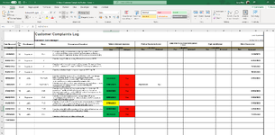
I've been trying to work this out for over a month! I have a spreadsheet that includes due dates for certain stages of a complaint.

Stage 1 must be actioned within 5 days of the due date, Stage 2 must be actioned within 10 days, Stage 3 is 30 days and Stage 4 is 56 days. The days need to exclude weekends and I've been tasked with making the cells change colours when the due date is nearing or overdue.

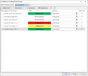
Currently I've been trialling these formulas within the <5 days stage: '=F6-TODAY()<=5' (No Formatting), '=F6-TODAY()<=3' (Yellow), '=F6-TODAY()<=5' (RED).

Then the 'Actioned' column has a formula that turns the date green once actioned and 'YES' is inputted into the next column.
I used the formula '=IF(G6="YES", TRUE,FALSE)' but even though I've made this apply to the G column, the G column still seems to go red, even with conditional formatting which specifies 'YES' as green.

I've also tried the '=WEEKDAY(F6)=5' but this doesn't appear to work, unless I'm using it wrong?

I've attached my rules and my spreadsheet (sorry, for some reason I couldn't attach it as the Mini-sheet)

Would anyone know a solution for this? I will be eternally grateful.

 

[Austin Lang]

Hi!

The order of rules in that list sets priority. I would move that rule up higher in the list with the carrot arrows in the top navigation bar. I suggest you move it above the rule that sets the red color. I also think you may want to remove the "Stop if true". That cause a hiccup too.

Hope this works.