Conditional formatting-format cell in column based on value in another cell (row by row)

[ljwisner]

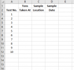
I am trying to format (bottom border) each cell in a column based on the value in the corresponding cell in the same row. I can do this individually to each cell, but would like the formatting to "read" the value in a cell, and format another accordingly for the entire column.

For example:


This is my workbook. I am trying to have a bottom border on cells B3-B12, C3-C12, D3-D12 based on the fact that cells A3-A12 have a number in them. I would like the bottom border of B12, C12, D12 to disappear if A12 does not have a number in it. Same goes for B11,C11,D11 if A11 doesn't have a number etc.

I can currently do this by selecting B2>conditional formatting>formula>=$A$2<>"".

I do not want to have to select each cell in the B,C,D columns to then "read" the corresponding A column cell.

Please help.

 

[ljwisner]

=COUNTA($A3:$Ax) will not work because there is a formula to determine if there is a number shown in column A

 

[Snakehips]

Try
Select the range B3:D12 > Cond Format > Formula > =ISNUMBER($A3)


Hope that helps

 

[ljwisner]

Try
Select the range B3:D12 > Cond Format > Formula > =ISNUMBER($A3)


Hope that helps

Thank you! This works. For some reason I completely forgot about ISNUMBER

 

[Peter_SSs]

Thank you! This works.

The marked solution has been changed accordingly. In your future questions, please mark the post as the solution that actually answered your question, instead of your feedback message as it will help future readers. No further action is required for this thread.