Conditional Formatting Finding Multiple Matched Values

[diderooy]

Hello,

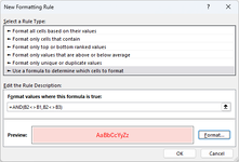
I have built a couple basic macros to convert some datasets from different sources to the same basic layout, where the lists of remaining values should each have a match within the other set. All the values should have an identical match, but I want to be able to isolate the ones that don't. I'm guessing I can use a COUNTIFS formula or something in the conditional formatting manager to achieve this, but I can't seem to get it right. Any ideas?

Here is a snip of a sample of my datasets, after I've combined them into the same table (on a new worksheet) and sorted them by column B:

I want to highlight rows where there is no match for column B or there is not a corresponding match in column C. With the first ticket as an example, I expect and found two rows of ticket # 10588019 with a matching weight of 45,340 lbs; if a keying error results in an "o" instead of a "0", I want it highlighted, if the weight is off by 10 lbs, I want it highlighted. Theoretically, I would see the following when I apply the conditional formatting rule:

Bear in mind, as seen in rows 2-5, there will be more than two rows with the same weight, but hopefully no more than 2 that correspond to the same ticket #.

 

[Joe4]

Do you mean like this?

As long as you have sorted your data by column B and column C, you could produce that result by selecting the range B2:C12, and entering in this Conditional Formatting formula:

=AND(B2<>B1,B2<>B3)

and choosing your desired formatting color.

 

[Joe4]

However, while the results of my previous post return the result you posted, I don't think that is really what you want, as it handles columns B and C independent on each other.
I think you want to take them in conjunction with one another, like this:

For that, you would still select range B2:C12, but use this Conditional Formatting formula instead:

=COUNTIFS($B:$B,$B2,$C:$C,$C2)=1

 

[diderooy]

The first of these appears to have accomplished what I was looking for, but does not display in the conditional formatting manager the way you indicated (or that I pasted). Why does the formula change from this:

to this:

after I click "OK" the first time?

If I manually change it back to the formula you gave, it will keep it, and then does not work. I'm sure I'm doing something wrong but I don't know what :/

 

[Joe4]

Do NOT select the whole column before entering the Conditional Formatting formula, since it is trying to look up one row. Start with row 2 and go down as far as you need/want, and then enter the formula.

 

[diderooy]

Oh, okay. In that case, the second formula (COUNTIF) does seem to work better.

Thank you for all your help! Happy Monday

 

[Joe4]

You are welcome.
Glad I was able to help!