Conditional formatting column with multiple conditions

[Metaphysix]

Trying to develop a single formula for conditional formatting that doesn't include a cell reference so I can apply to an entire column. My data is a column of dates, but runs across multiple blanks and column headers that I don't want formatted.

Conditions:

1. not(isblank)
2. is(date)
3. <today() +7

I was able to sort of get these conditions checked when using cell references, but having a hard time translating this into a format that could be applied as a true / false test for each cell in a column:

=AND(A1<>"",IF(LEFT(CELL("format",A1),1)="D","TRUE","FALSE"),A1<TODAY()+7)

Probably a simpler way to get the date format checked, but this works. Also need to double check that the AND statement evaluates the result from the 2nd logic test as TRUE / FALSE rather than text, but it seems to work so far.

Any help would be appreciated!

 

[DanteAmor]

Try:

Dante Amor
	A
1	Date
2	10-nov
3	11-nov
4	12-nov
5	13-nov
6	14-nov
7	15-nov
8	16-nov
9	17-nov
10	18-nov
11	19-nov
12	20-nov
13	21-nov
Sheet1

Cells with Conditional Formatting
Cell	Condition		Cell Format	Stop If True
A2:A13	Expression	=Y(A2<>"",CELDA("format",A2)="D2",A2<HOY()+7)	text	NO

 

[Metaphysix]

Thanks, I'm not familiar with the CELDA or HOY functions and they don't seem to be recognized when I try to build a formula outside of conditional formatting, but it is accepting that as a valid formula. Wish there was a way to view syntax and evaluate the formula when working in conditional formatting.

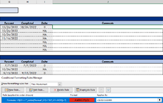
Unfortunately, I'm not getting any indication that the formula is working. I changed all the "A1" references to "G1" where my source data lives, and have run through D1 / D2 / D3 / D4 as possible outputs for date formatting, but none seem to be triggering the condition. Next steps?

 

[DanteAmor]

Sorry. It's my fault. My excel is in Spanish.

According to your image your dates start in cell G6. So the conditional formatting must start in cell G6

The corrected formula:

Dante Amor
	G
5	FECHA
6	10-nov
7	11-nov
8	12-nov
9	13-nov
10	14-nov
11	15-nov
12	16-nov
13	17-nov
14	18-nov
15	19-nov
16	20-nov
17	21-nov
Sheet1

Cells with Conditional Formatting
Cell	Condition		Cell Format	Stop If True
G6:G17	Expression	=AND(G6<>"",CELL("format",G6)="D2",G6<TODAY()+7)	text	NO