Conditional Formatting and '=IF' help?

[mcooper22]

Hi All,

Appreciate any help with this and my limited excel knowledge.

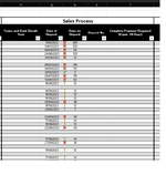
Currently using conditional formatting if the cell in R has a value below 7 it's okay and a green tick, above 7 and below 21 it's amber, above 21 it's a red X

What I would like to do, is keep it doing that, however if there is a deposit number in S column it negates the need for the formatting in column R.

Furthermore, if there is a date of deposit in column Q - then column T will have 21 days from that date before it becomes highlighted in Red (I assume I can just do that in conditional formatting)

If that at all is possible, it would be fantastic, and any help would be appreciated.

 

[awoohaw]

Try this for column R, I'm assuming you have Q covered.
(Note: The formatting of Icon Sets did not copy, so there is an image)

Mr Excel Questions 71.xlsm
	P	Q	R	S	T	U
1
2	Terms & Bank Details Sent	Date of Deposit	Days on Deposit	Deposit Number	Formatting R	=IF(S3<>"","Skip Formatting",IF(R3<7,"Ok Green Tick",IF(R3<21,"Amber Tick","Red X")))
3		2023-10-01	30	54	Skip Formatting
4		2023-10-04	27	65	Skip Formatting
5		2023-10-07	24		Red X
6		2023-10-10	21		Red X
7		2023-10-13	18		Amber Tick
8		2023-10-16	15		Amber Tick
9		2023-10-19	12		Amber Tick
10		2023-10-22	9		Amber Tick
11		2023-10-25	6		Ok Green Tick
12		2023-10-28	3		Ok Green Tick
13		2023-10-31	0		Ok Green Tick
mcooper22

Cell Formulas
Range	Formula
U2	U2	=FORMULATEXT(T3)
Q3	Q3	=DATE(2023,10,1)
R3:R13	R3	=TODAY()-Q3
Q4:Q13	Q4	=Q3+3
T3:T12	T3	=IF(S3<>"","Skip Formatting",IF(R3<7,"Ok Green Tick",IF(R3<21,"Amber Tick","Red X")))
T13	T13	=IF(S13<>"",FALSE,IF(R13<7,"Ok Green Tick",IF(R13<21,"Amber Tick","Red X")))

Cells with Conditional Formatting
Cell	Condition		Cell Format	Stop If True
R3:R13	Expression	=S3<>""	text	YES
R3:R13	Other Type	Icon set		NO