Complex lookup formula for simple Data Validation

[HScott22]

Hello,

I am comparing 2 files for direct deposit data validation. I want to compare that the files match (All columns and rows).

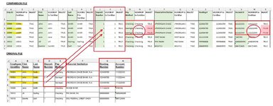
The files are basic. But here lies the problem...some employees have multiple lines of direct deposit accounts and it only looks at their first line and then populates the compare with only the first line.

Picture attached:
I have a compare file with the ORIGINAL data and Vlookup <<<(=VLOOKUP(A2,Ceridian!A:A,1,0)>>> pulls the data to compare into the same sheet. Then there is a simple = formula to show any difference.

 

[Eric W]

Welcome to the MrExcel forum!

I believe I got the gist of your query, although I had trouble with some of the details. I think the overall idea is that if there are multiple rows with the same EMP ID in it, then the nth instance of that EMP ID should return the nth instance from the lookup table?

If so, consider these sheets:

Book2
	A	B	C	D	E	F	G	H
1	Emp ID	First Name	Last Name	Deposit Number	Pay Method	Financial Institution	Routing Number	Account Number
2	10004	John	Smith	1	Checking	JPMORGAN CHASE BANK, N.A.	123456789	111222333
3	10004	John	Smith	2	Savings1	JPMORGAN CHASE BANK, N.A.	123456789	111222444
4	10004	John	Smith	3	Savings2	JPMORGAN CHASE BANK, N.A.	123456789	111222555
5
Original

Book2
	A	B	C	D	E	F	G	H	I	J	K	L	M	N	O	P	Q	R	S	T	U	V	W	X
1	Emp ID	LOOKUP	Match?	First Name	LOOKUP	Match?	Last Name	LOOKUP	Match?	Deposit Number	LOOKUP	Match?	Pay Method	LOOKUP	Match?	Financial Institution	LOOKUP	Match?	Routing Number	LOOKUP	Match?	Account Number	LOOKUP	Match?
2	10004	10004	TRUE	John	John	TRUE	Smith	Smith	TRUE	1	1	TRUE	Checking	Checking	TRUE	JPMORGAN CHASE BANK, N.A.	JPMORGAN CHASE BANK, N.A.	TRUE	123456789	123456789	TRUE	111222333	111222333	TRUE
3	10004	10004	TRUE	John	John	TRUE	Smith	Smith	TRUE	1	2	FALSE	Savings1	Savings1	TRUE	JPMORGAN CHASE BANK, N.A.	JPMORGAN CHASE BANK, N.A.	TRUE	123456789	123456789	TRUE	111222444	111222444	TRUE
4	10004	10004	TRUE	John	John	TRUE	Smith	Smith	TRUE	1	3	FALSE	Savings2	Savings2	TRUE	JPMORGAN CHASE BANK, N.A.	JPMORGAN CHASE BANK, N.A.	TRUE	123456789	123456789	TRUE	111222555	111222555	TRUE
Comparison

Cell Formulas
Range	Formula
B2:B4	B2	=INDEX(FILTER(Original!$A$2:$A$1000,Original!$A$2:$A$1000=A2,"No match"),COUNTIFS(A$2:A2,A2))
C2:C4,X2:X4,U2:U4,R2:R4,O2:O4,L2:L4,I2:I4,F2:F4	C2	=A2=B2
E2:E4,W2:W4,T2:T4,Q2:Q4,N2:N4,K2:K4,H2:H4	E2	=LET(v,INDEX(Original!$A$2:$H$1000,0,MATCH(D$1,Original!$A$1:$H$1,0)),f,FILTER(v,Original!$A$2:$A$1000=$A2),INDEX(f,COUNTIFS($A$2:$A2,$A2)))

Cells with Conditional Formatting
Cell	Condition		Cell Format	Stop If True
A1:X4	Expression	=A1=FALSE	text	NO

To make the formula simpler, I made the headings on both sheets match. If that's a problem, you can hard code the column number in the each formula.

Also, as an FYI, look into the xl2bb add-in (see the link in the reply box). It allows you to display your data in a way that lets the helpers here copy it, and not have to retype everything from a picture. You're likely to get faster results if you use it.

Anyway, let us know if this works for you.

 

[HScott22]

You sir are a life saver!

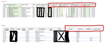
It has worked AMAZING for my first several columns of data, but not my last 4 even when I tried to edit the formula. Its still showing N/A (my edits are below).

I am crossing my fingers to learn as much about this formula as I can to use in other data validations.

1. Columns need to have the same title
2. what else should I note?


**I am not able to use the xl2bb add in. I am on my work computer. I will actually try to use my personal and load that for any further posts.


My Formula Edits:
For each formula I edited the column it was looking at (See RED below)
Account #:
=LET(v,INDEX(Original!$A$2:$H$1000,0,MATCH(V$1,Original!$A$1:$H$1,0)),f,FILTER(v,Original!$A$2:$A$1000=$A2),INDEX(f,COUNTIFS($A$2:$A2,$A2)))


Deposit Value:
=LET(v,INDEX(Original!$A$2:$H$1000,0,MATCH(Y$1,Original!$A$1:$H$1,0)),f,FILTER(v,Original!$A$2:$A$1000=$A2),INDEX(f,COUNTIFS($A$2:$A2,$A2)))

Deposit Type
=LET(v,INDEX(Original!$A$2:$H$1000,0,MATCH(AB$1,Original!$A$1:$H$1,0)),f,FILTER(v,Original!$A$2:$A$1000=$A2),INDEX(f,COUNTIFS($A$2:$A2,$A2)))


Requires Pre Note:
=LET(v,INDEX(Original!$A$2:$H$1000,0,MATCH(AE$1,Original!$A$1:$H$1,0)),f,FILTER(v,Original!$A$2:$A$1000=$A2),INDEX(f,COUNTIFS($A$2:$A2,$A2)))

 

[Eric W]

Change the green H in all the formulas below to L. The ranges in the formulas must match the full table in the Original sheet, which stretches to L. If you still have trouble, double check that the headings match exactly, no extra spaces.

Account #:
=LET(v,INDEX(Original!$A$2:$H$1000,0,MATCH(V$1,Original!$A$1:$H$1,0)),f,FILTER(v,Original!$A$2:$A$1000=$A2),INDEX(f,COUNTIFS($A$2:$A2,$A2)))
Deposit Value:
=LET(v,INDEX(Original!$A$2:$H$1000,0,MATCH(Y$1,Original!$A$1:$H$1,0)),f,FILTER(v,Original!$A$2:$A$1000=$A2),INDEX(f,COUNTIFS($A$2:$A2,$A2)))
Deposit Type
=LET(v,INDEX(Original!$A$2:$H$1000,0,MATCH(AB$1,Original!$A$1:$H$1,0)),f,FILTER(v,Original!$A$2:$A$1000=$A2),INDEX(f,COUNTIFS($A$2:$A2,$A2)))
Requires Pre Note:
=LET(v,INDEX(Original!$A$2:$H$1000,0,MATCH(AE$1,Original!$A$1:$H$1,0)),f,FILTER(v,Original!$A$2:$A$1000=$A2),INDEX(f,COUNTIFS($A$2:$A2,$A2)))