Colored cells operations

[Antonescu]

Hey, guys,

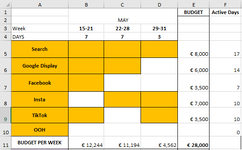
Could you please give me a hand with something. I am making a media plan and want to calculate the spend per week. The way it works is: I have multiple channels, spread by weeks and each channel has a budget. The days when I communicate through that channel, I manually color the cell (please see attached photo for the colored plan).

What I have is:

• With the kind help of @Fluff, the VBA Code for the colored cells

Function IsCellColored(CellRange As Range) As Variant
Dim Result() As Variant
ReDim Result(1 To 1, 1 To CellRange.Cells.Count)
Dim i As Integer
i = 1
For Each rCell In CellRange
Result(1, i) = (rCell.Interior.ColorIndex <> xlNone)
i = i + 1
Next rCell
IsCellColored = Result
End Function

The desired outcome:

• Budget per week, for cells B11, C11, D11. Now they are added manually. What it should be is something the likes of: B11 = SUM of IF IsCellColored(B5:B10), E5:E10 / F5:F10 * C4. Basically, the SUM of (BUDGET / active days * days in the week) for all the active channels in that week, but of course, only for the colored cells.

Thank you very much!

	MAY			BUDGET	Active Days
Week	15-21	22-28	29-31
DAYS	7	7	3
Search				€ 8,000	17
Google Display				€ 6,000	14
Facebook				€ 3,500	7
Insta				€ 7,000	10
TikTok				€ 3,500	10
OOH					0
BUDGET PER WEEK	€ 12,244	€ 11,194	€ 4,562	€ 28,000

 

[sijpie]

I have rewritten your IsCellColored function to give the result in an array with the same number of rows and columns as the input range.
Then it is easy to make a second function, where only those cells are summed whre the corresponding cell in the array is true

Option Explicit



Function IsCellColored(CellRange As Range) As Variant
    Dim Result() As Variant
    Dim rCell As Range
    ReDim Result(1 To CellRange.Rows.Count, 1 To CellRange.Columns.Count)
    For Each rCell In CellRange
        Result(rCell.Row - CellRange.Row + 1, rCell.Column - CellRange.Column + 1) = (rCell.Interior.ColorIndex <> xlNone)
    Next rCell
    IsCellColored = Result
End Function



Function SumColoured(CellRange As Range) As Double
    Dim vUse As Variant
    Dim lR As Long, lC As Long, UB1 As Long, UB2 As Long
    
    UB1 = CellRange.Rows.Count
    UB2 = CellRange.Columns.Count
    
    vUse = IsCellColored(CellRange)
    
    For lR = 1 To UB1
        For lC = 1 To UB2
            If vUse(lR, lC) Then
                SumColoured = SumColoured + CellRange(lR, lC)
            End If
        Next lC
    Next lR
    
End Function

 

[sijpie]

Oh, yes: next time when you post code, do it in between code brackets. You should know this by now.

 

[Antonescu]

Oh, yes: next time when you post code, do it in between code brackets. You should know this by now.

Thanks for the help! I don't doubt it's correct, however I couldn't verify it since it's exactly that final formula that I can't get right, which is the subject of this post. And, I apologize, I literally had no idea that code goes is brackets or how I should have had this information by now. This is the 3rd time ever I use code, and you're the first to mention this. But I will keep in mind, thanks!

 

[sijpie]

I will have a look at it. I see I forgot to read your post properly.

 

[sijpie]

Writing this UDF is more difficult than I expected: The reason is that one can't Range.Currentregion in a UDF (to be used in a spreadsheet).

So you will have to pass TWO ranges to the function: one is the range (column) with coloured cells, the other is the range holding the budget and active days.

mei23.xlsm
	A	B	C	D	E	F
1		May			Budget	Active Days
2
3	Week	15-21	22-28	29-31
4	Days	7	7	3
5	a				8000	17
6	b				5000	14
7	c				12000	7
8	d				4000	10
9	e				5000	10
10	f					0
11	budget per week	8594.12	17300.00	4111.76
Sheet9

Cell Formulas
Range	Formula
B11:D11	B11	=SumBudgetColoredCells(B5:B10,$E$5:$F$10)

The vba code for the UDF:

Option Explicit

Function IsCellColored(CellRange As Range) As Variant
    Dim Result() As Variant
    Dim rCell As Range
    ReDim Result(1 To CellRange.Rows.Count, 1 To CellRange.Columns.Count)
    For Each rCell In CellRange
        Result(rCell.Row - CellRange.Row + 1, rCell.Column - CellRange.Column + 1) = (rCell.Interior.ColorIndex <> xlNone)
    Next rCell
    IsCellColored = Result
End Function


Function SumBudgetColoredCells(rColRange As Range, rBudgActD As Range) As Double
    Dim vUse As Variant, vBA As Variant
    Dim lR As Long, lC As Long, UB1 As Long, UB2 As Long, _
        lROffs As Long, lCOffs As Long, lSt As Long, lCBudg As Long, lCActD As Long
    Dim rDay As Range
    
    ' get row of DAY
    Set rDay = Range("A:A").Find(what:="DAYS")
    If Not rDay Is Nothing Then
        Set rDay = rDay.Offset(0, rColRange.Column - 1)
        Debug.Print rDay.Value
        
        UB1 = rColRange.Rows.Count
        UB2 = rColRange.Columns.Count
        
        vUse = IsCellColored(rColRange)
        For lR = 1 To UB1
            For lC = 1 To UB2
                If vUse(lR, lC) Then
                    SumBudgetColoredCells = SumBudgetColoredCells + (rBudgActD(lR, 1) / rBudgActD(lR, 2)) * rDay.Offset(0, lC - 1).Value
                End If
            Next lC
        Next lR
    Else
        SumBudgetColoredCells = Error(1)
    End If
        
End Function

The code is a bit rough. it does not check if the two ranges have the same number of rows for instance.