Change cell color based on the number in the cell

[rplohocky]

Hello,
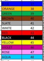
I would like to use either conditional formatting, a macro or another method to make a cell(s) turn a specific color based on what number is in a specific cell. An example would be if cell D3 = 1, 13, 25, 37, 49, 61, 73, 84, 97, 109, 121 or 133 then turn cells C and D BLUE. I need this for 12 colors.
List:
if cell D3 = 1, 13, 25, 37, 49, 61, 73, 84, 97, 109, 121 or 133 then turn cells C and D BLUE. (EACH NUMBER IS UNIQUE TO EACH COLOR)
if cell D3 = 2, 14, 26, 38, 50, 62, 74, 85, 98, 110, 122 or 134 then turn cells C and D ORANGE.
if cell D3 = 3, 15, 27, 39, 51, 63, 75, 86, 99, 111, 123 or 135 then turn cells C and D GREEN.
if cell D3 = 4, 16, 28, 40, 52, 64, 76, 87, 100, 112, 124 or 136 then turn cells C and D BROWN.
if cell D3 = 5, 17, 29, 41, 53, 65, 77, 88, 101, 113, 125 or 137 then turn cells C and D SLATE.
if cell D3 = 6, 18, 30, 42, 54, 66, 78, 89, 102, 114, 126 or 138 then turn cells C and D WHITE.

 

[etaf]

select your range you want coloured

Lets Assumme Column C3 to D100
then select C3 to D100 - NOTE the row in the selection thats starts would need to also be used in the formula

SO as you are using row 3 as the starting point

Select a new Rule for each of the formula for each of the colours

You cannot use arrays in Conditional Formatting then an OR with the numbers OR a table list for each colour and a COUNTIF() =1

if cell D3 = 1, 13, 25, 37, 49, 61, 73, 84, 97, 109, 121 or 133 then turn cells C and D BLUE. (EACH NUMBER IS UNIQUE TO EACH COLOR)
OR ( $D3 =1, $D3 =13, $D3 =25, $D3 =37,$D3 = 49, $D3 =61, $D3 =73,$D3 = 84, $D3 =97, $D3 =109, $D3 =121 ,$D3 = 133 )
Set fill colour for these
New RULE

if cell D3 = 2, 14, 26, 38, 50, 62, 74, 85, 98, 110, 122 or 134 then turn cells C and D ORANGE.
OR( $D3 = 2, $D3 =14,$D3 = 26, $D3 =38, $D3 =50, $D3 =62, $D3 =74, $D3 =85, $D3 =98, $D3 =110, $D3 =122 ,$D3 =134 )
Set fill colour for these
New RULE

if cell D3 = 3, 15, 27, 39, 51, 63, 75, 86, 99, 111, 123 or 135 then turn cells C and D GREEN.
OR ( $D3 = 3, $D3 =15, $D3 =27, $D3 =39, $D3 =51, $D3 =63, $D3 =75, $D3 =86, $D3 =99,$D3 = 111,$D3 = 123 ,$D3 = 135)
Set fill colour for these
New RULE

if cell D3 = 4, 16, 28, 40, 52, 64, 76, 87, 100, 112, 124 or 136 then turn cells C and D BROWN.
OR ( $D3 =4, $D3 =16, $D3 =28, $D3 =40,$D3 = 52, $D3 =64, $D3 =76,$D3 = 87, $D3 =100,$D3 = 112, $D3 =124 ,$D3 =136)
Set fill colour for these
New RULE

if cell D3 = 5, 17, 29, 41, 53, 65, 77, 88, 101, 113, 125 or 137 = then turn cells C and D SLATE.
OR( $D3 =5, $D3 =17, $D3 =29, $D3 =41, $D3 =53, $D3 =65, $D3 =77,$D3 = 88, $D3 =101,$D3 = 113, $D3 =125 ,$D3 = 137)
Set fill colour for these
New RULE

if cell D3 = 6, 18, 30, 42, 54, 66, 78, 89, 102, 114, 126 or 138 then turn cells C and D WHITE.
OR( $D3 = 6, $D3 =18,$D3 = 30,$D3 = 42,$D3 = 54,$D3 = 66, $D3 =78, $D3 =89, $D3 =102,$D3 = 114,$D3 = 126 , $D3 =138)
Set fill colour for these
New RULE

OR use
COUNTIF( Table with that colours numbers in , $D3 ) =1
I Table for each of the colours and 1 rule

 

[Fluff]

Assuming that the numbers in the 80s are wrong & should be 85,86 etc, & not 84,85 etc try

+Fluff 1.xlsm
	C	D
1
2
3		1
4		2
5		3
13		11
14		12
15		13
16		14
17		15
25		23
26		24
27		25
28		26
29		27
37		35
38		36
39		37
40		38
41		39
49		47
50		48
51		49
52		50
53		51
61		59
62		60
63		61
64		62
65		63
73		71
74		72
75		73
76		74
77		75
85		83
86		84
87		85
88		86
89		87
90		88
Master

Cells with Conditional Formatting
Cell	Condition		Cell Format	Stop If True
C3:D140	Expression	=MOD($D3-3,12)=0	text	NO
C3:D140	Expression	=MOD($D3-2,12)=0	text	NO
C3:D140	Expression	=MOD($D3-1,12)=0	text	NO

 

[etaf]

i have as an example just show the table and countif with 3 formulas as an example here

Book1
	C	D	E	F	G	H	I	J	K	L	M	N	O	P	Q
2										BLUE.	ORANGE.	GREEN.	BROWN.	SLATE.	WHITE.
3		1								1	2	3	4	5	6
4		2								13	14	15	16	17	18
5		3								25	26	27	28	29	30
6		1								37	38	39	40	41	42
7		1								49	50	51	52	53	54
8		2								61	62	63	64	65	66
9		2								73	74	75	76	77	78
10		3								84	85	86	87	88	89
11		3								97	98	99	100	101	102
12		3								109	110	111	112	113	114
13		2								121	122	123	124	125	126
14		3								133	134	135	136	137	138
15		3
16		2
17		1
Sheet1

Cells with Conditional Formatting
Cell	Condition		Cell Format	Stop If True
C3:D24	Expression	=COUNTIF($N$3:$N$14,$D3)=1	text	NO
C3:D24	Expression	=COUNTIF($M$3:$M$14,$D3)=1	text	NO
C3:D24	Expression	=COUNTIF($L$3:$L$14,$D3)=1	text	NO

 

[jtakw]

Hi,

Select the cells you want CF.

Use this formula:

=AND($D3>0,$D3<=144,MOD($D3,12)=1)

Change the 1 at the end of the formula to 2, 3, 4, etc. up to 12 for Each of your 12 different colors.

Book3.xlsx
	D	E	F	G	H	I								Q	R	S	T	U	V
3	-11	2	3	4	5	6								FALSE	TRUE	TRUE	TRUE	TRUE	TRUE
4	13	14	15	16	17	18								TRUE	TRUE	TRUE	TRUE	TRUE	TRUE
5	25	26	27	28	29	30								TRUE	TRUE	TRUE	TRUE	TRUE	TRUE
6	37	38	39	40	41	42								TRUE	TRUE	TRUE	TRUE	TRUE	TRUE
7	49	50	51	52	53	54								TRUE	TRUE	TRUE	TRUE	TRUE	TRUE
8	61	62	63	64	65	66								TRUE	TRUE	TRUE	TRUE	TRUE	TRUE
9	73	74	75	76	77	78								TRUE	TRUE	TRUE	TRUE	TRUE	TRUE
10	85	86	87	88	89	90								TRUE	TRUE	TRUE	TRUE	TRUE	TRUE
11	97	98	99	100	101	102								TRUE	TRUE	TRUE	TRUE	TRUE	TRUE
12	109	110	111	112	113	114								TRUE	TRUE	TRUE	TRUE	TRUE	TRUE
13	121	122	123	124	125	126								TRUE	TRUE	TRUE	TRUE	TRUE	TRUE
14	133	134	135	136	137	138								TRUE	TRUE	TRUE	TRUE	TRUE	TRUE
15	145	146	147	148	149	150								FALSE	FALSE	FALSE	FALSE	FALSE	FALSE
Sheet890

Cell Formulas
Range	Formula
Q3:Q15	Q3	=AND($D3>0,$D3<=144,MOD($D3,12)=1)
R3:R15	R3	=AND($E3>0,$E3<=144,MOD($E3,12)=2)
S3:S15	S3	=AND($F3>0,$F3<=144,MOD($F3,12)=3)
T3:T15	T3	=AND($G3>0,$G3<=144,MOD($G3,12)=4)
U3:U15	U3	=AND($H3>0,$H3<=144,MOD($H3,12)=5)
V3:V15	V3	=AND($I3>0,$I3<=144,MOD($I3,12)=6)

 

[jtakw]

Use this formula:

=AND($D3>0,$D3<=144,MOD($D3,12)=1)

Change the 1 at the end of the formula to 2, 3, 4, etc. up to 12 for Each of your 12 different colors.

Oops, the above underlined part should say 0 (zero), Not 12, so

Change the 1 at the end of the formula to 2, 3, 4, etc. up to 11, then use 0 for the 12th color, for Each of your 12 different colors.

Let me know if you need further explanation.