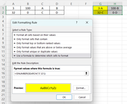
Can a Conditional Formula highlight cell G2 in range (G1:H2) that contains value 32? Where two cells values are combined into one cell?

[arthurz11]

 

[Fluff]

How about

=ISNUMBER(SEARCH(" 32-"," "&G1))

 

[dreid1011]

Yes, CF can do that.

Book1
	A	B	C	D	E	F	G	H
1	1	100	A	B			1-A	100-B
2	32	0	C	D			32-C	0-D
Sheet1

Cells with Conditional Formatting
Cell	Condition		Cell Format	Stop If True
G1:H2	Expression	=ISNUMBER(SEARCH("32",G1))	text	NO

 

[arthurz11]

Yes, CF can do that.

Book1
	A	B	C	D	E	F	G	H
1	1	100	A	B			1-A	100-B
2	32	0	C	D			32-C	0-D
Sheet1

Cells with Conditional Formatting
Cell	Condition		Cell Format	Stop If True
G1:H2	Expression	=ISNUMBER(SEARCH("32",G1))	text	NO

It didn't quite worked. Notice I changed the cell A1 value to 3. Using the conditional formula that you wrote, it now highlights cell G1 and G2. Both cells have a number 3. So the formula checks to see if it has a 3. Weather it's 3,000, 300, 32, or a 3 it is highlighted. How can I revised your formula so it will only highlight cell G2 that has the value 32, even it there's another cell that has a 3 value?

 

[Fluff]

Did you try the formula I suggested?

 

[dreid1011]

It didn't quite worked. Notice I changed the cell A1 value to 3. Using the conditional formula that you wrote, it now highlights cell G1 and G2. Both cells have a number 3. So the formula checks to see if it has a 3. Weather it's 3,000, 300, 32, or a 3 it is highlighted. How can I revised your formula so it will only highlight cell G2 that has the value 32, even it there's another cell that has a 3 value?

I see the formula you are actually using is only searching for "3" and not "32", but perhaps give Fluff's formula a try as it will only highlight 32, and not any larger numbers that have 32 in them.

Did you try the formula I suggested?

 

[arthurz11]

I doubled check to be certain. I used this one =ISNUMBER(SEARCH(" 32-"," "&G1)) and nothing was highlighted. Then I used someone elses formula =ISNUMBER(SEARCH("32",G1)) and it highlighted cell G2. But when I changed cell A1 to 3 the formula =ISNUMBER(SEARCH("3",G1)) highlighted cells G1 and G2

 

[Fluff]

I used this one =ISNUMBER(SEARCH(" 32-"," "&G1)) and nothing was highlighted

It works for me.

Fluff.xlsm
	A	B	C	D	E	F	G	H
1	3	321	A	B			3-A	321-B
2	32	132	C	D			32-C	132-D
Data

Cell Formulas
Range	Formula
G1:H2	G1	=A1&"-"&C1

Cells with Conditional Formatting
Cell	Condition		Cell Format	Stop If True
G1:H2	Expression	=ISNUMBER(SEARCH(" 32-"," "&G1))	text	NO

 

[dreid1011]

I doubled check to be certain. I used this one =ISNUMBER(SEARCH(" 32-"," "&G1)) and nothing was highlighted. Then I used someone elses formula =ISNUMBER(SEARCH("32",G1)) and it highlighted cell G2. But when I changed cell A1 to 3 the formula =ISNUMBER(SEARCH("3",G1)) highlighted cells G1 and G2

Changing the value in A1 shouldn't have changed the CF formula. So I can only imagine you had =ISNUMBER(SEARCH("3",G1)) the whole time and didn't notice.

 

[arthurz11]

Sorry for the very late reply. It's even more frustrated trying to solve it and just having a tooth extracted. (for real). Just got back from the dentist. Anyway, I removed the text (letters) from the cells so I can explain myself more clearly. I used only numeric values. I just want to highlight the number 3 (“first value” before the hyphen) Or just want to highlight the number 32 (“first value” before the hyphen) Please view the image.