Basic VLOOKUP Formula

[Apples52]

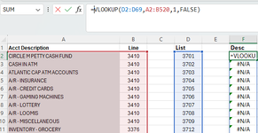
I'm needing help with what I think is a very basic vlookup formula. In column F, I want the description from column A returned if a value from the List column D appears in the column B. Can't figure out where I'm going wrong with this simple formula.

 

[hagia_sofia]

Without some tunning, VLOOKUP is not able to search to the left - is it possible for you to switch those columns (i.e. A - B) or would you prefer a formula to enable that?

 

[Apples52]

Without some tunning, VLOOKUP is not able to search to the left - is it possible for you to switch those columns (i.e. A - B) or would you prefer a formula to enable that?

In this case, yes it's easy enough for me to switch those colmuns. I moved these to columns H and I with a simple = formula. I then tried the vlookup formula in column K and it picked up some, but its not picking up everything. It stops at row 69, which is how long my list is in column D, but the data I want it to search through in columns H and I are much longer.

 

[Cubist]

Make sure your data types in col D and H match i.e. both text or numeric.

 

[Apples52]

Make sure your data types in col D and H match i.e. both text or numeric

I had made sure they were both "general" before. Tried changing to both text and number, but neither worked. My column K still stops at row 69 instead of continuing to the end of columns H and I. They end 321, so some of the data that should match isn't getting picked up.

 

[Cubist]

I had made sure they were both "general" before. Tried changing to both text and number, but neither worked. My column K still stops at row 69 instead of continuing to the end of columns H and I. They end 321, so some of the data that should match isn't getting picked up.

Formatting doesn't tell you what the stored data type is. Try =ISNUMBER(cell) or =ISTEXT(cell).

 

[Apples52]

Formatting doesn't tell you what the stored data type is. Try =ISNUMBER(cell) or =ISTEXT(cell).

I tried both of those formulas in a new column and there were some differences. With =ISNUMBER, there were some cells that had text in them and I deleted those rows because I didnt need those specific ones. Everything says TRUE with the =ISNUMBER check, but the results are still stopping at row 69 as in my second attachment.

 

[Cubist]

Try:

=VLOOKUP(--D1:D69,--H1:I500,2,FALSE)

 

[Alex Blakenburg]

I think we need better description of what you are trying to do.

Based on the current description and formula what the VLookup is going to do is look at each value in the range D1:D69 and find the first matching value in the range H1:H500 returning the Value from I1:I500, so it will perform 69 lookups returning 69 values (or #N/A)
Even this shouldn't work in Excel 2019, is your Account Profile actually correct ? What version are you using and if not 2019 please update your profile.

You seem to be expecting multiple return values for each lookup, is that the case ?