AverageIfs exclude zeros

[Sherm]

Hello,

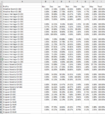
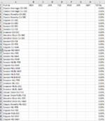
I am looking to average a massive set of data for a specific profile and look it up onto another tab, basically a sumifs but I want the average instead. I am using the formula AverageIfs which is working just fine and getting me to 100%, BUT then I realized it is including zeros which is throwing off what the average should really be. How do I do an AverageIFs that excludes zeros but also gets me to 100%. So in the first table I want to average all the %s in column "11" (there are like 1,800 rows so more than what is shown), and enter that average in the second table under NOV. I have used the "<>0" in my formula but the when I add up NOV - MAY it doesn't equal 100%. Is this even possible? First time posting on forum so sorry if this doesn't make sense!

Little background: I am averaging the units sold per month from month 11-5. So for all the "Weather Boot-CO-DEC" in the 1,800 rows, I want that total average, which I am looking up into another tab.

Planning Category-Project Type-Atlas Month	11	12	1	2	3	4	5	Total
Weather Boot-CO-DEC	0.00%​	13.38%​	31.86%​	36.06%​	8.89%​	6.51%​	3.29%​	100.00%​
Weather Boot-CO-DEC	0.00%​	13.66%​	27.70%​	43.87%​	7.02%​	4.77%​	2.98%​	100.00%​
Classic Heritage-CO-DEC	0.00%​	59.68%​	11.39%​	21.47%​	7.46%​	0.00%​	0.00%​	100.00%​
Classic Heritage-CO-DEC	0.00%​	56.85%​	17.77%​	12.86%​	10.79%​	0.00%​	1.72%​	100.00%​
Classic Heritage-CO-DEC	0.00%​	73.93%​	8.93%​	13.58%​	1.82%​	1.37%​	0.36%​	100.00%​

Profile	NOV	DEC	JAN	FEB	MAR	APR	MAY	TOTAL
Classic Heritage-CO-DEC								0.00%​
Classic Heritage-CU-DEC								0.00%​
Classic Novelty-CO-DEC								0.00%​
Classic Novelty-CU-DEC								0.00%​
Slipper-CO-DEC								0.00%​
Slipper-CU-DEC								0.00%​
Sandal-CO-DEC								0.00%​
Sandal-CU-FEB								0.00%​
Sneaker-CO-DEC								0.00%​
Weather Boot-CO-DEC								0.00%​
Weather Boot-CU-DEC								0.00%​
Sandal-CO-FEB								0.00%​
Slipper-CO-FEB								0.00%​

 

[Joe4]

Welcome to the Board!

You should be able to use AVERAGEIFS, with the criteria of "<>0".
Can you post the actual formula that you are trying?

Also, I am a bit confused as to what you expect for an answer.
Depending on what exactly you are trying to average, the averages may not add up to zero (if the issue is it is off by tiny amount, like 0.01%, that is to be expected).

I think it would be best to post a real small data example that illustrates your problem, showing us what you expect for an answer, and what you are actually getting.

 

[Sherm]

Thanks for the advice! I'll try to be more clear. Also as you stated, not sure if this is even possible.

In the photo below 'Profile Lookup" I want the average of column B for the specific Profile in Column A and I want to enter that average into Column B in the 'Final Profile' picture. I don't want to include the zeros because that would change the average because it would include the zeros in the total number it's dividing by.

So if I have 100 cells its trying to average but only 5 of them are greater than 0, that makes a difference. If the total of the 100 cells is 87 lets say, 87/100 cells is going to give you a different average than 87/5 cells that are greater than 0.

 

[Joe4]

Because each column may have a different number of zeroes, you might be dividing each colunn by a different count, so it is quite possible that the total of the averages may NOT equal to 100%.
That is to be expected.

This can be illustrated in a simple example. Here is a small sample of 3 records, with 0's interspersed:

Planning Category-Project Type-Atlas Month	11​	12​	1​	2​	3​	4​	5​	Total
Classic Heritage-CO-DEC	0.00%​	20.00%​	20.00%​	20.00%​	20.00%​	20.00%​	0.00%​	100.00%​
Classic Heritage-CO-DEC	0.00%​	0.00%​	0.00%​	50.00%​	30.00%​	0.00%​	20.00%​	100.00%​
Classic Heritage-CO-DEC	0.00%​	0.00%​	10.00%​	30.00%​	40.00%​	10.00%​	10.00%​	100.00%​

And this is what the average of each would look like (you can clickly manually verify this):

Averages	11​	12​	1​	2​	3​	4​	5​	Total
Classic Heritage-CO-DEC	0.00%​	20.00%​	15.00%​	33.33%​	30.00%​	15.00%​	15.00%​	128.33%​

You can see that each monthly average is correct, and the Total does not add up to 100%.
That is because not all months have the same number of zeroes, so you are kind of creating "weighted averages".

 

[Sherm]

Thank you, that was what I was thinking might be the case.