AND conditional formatting

[LindaLinda]

Hello,
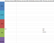
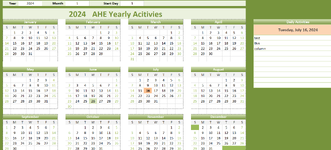
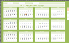
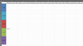
I'm trying to conditionally format when the date value in any cell in a range matches the date value of any cell in another range AND if cells in the corresponding with those date ranges are not blank.
currently I have =AND(B7:AF30='2024'B1:NC1,'2024'B20:NC25<>"") which is not working. See pictures for reference.
Please help!

 

[Jeffrey Mahoney]

This is an important part of CF formulas.
* The formula must test the TOP LEFT Cell in the range you want to affect. So if the CF range is A1:A10, then you are using A1 as your cell to compare.
* You cannot compare that to many cells

Since there are no column headers in your pictures, I can't tell what your CF range is. IF B7:AF30 is your CF range, then =AND(B7='2024'B1,B7<>"") might be the correct formula

 

[LindaLinda]

Thank you for this. After thinking about this a bit more, I believe the formula may actually be simpler. I believe it might be just an IF statement.
=IF('2024'!B20:B25<>"") then highlight the cell on the Activities Calendar that corresponds to the value in row 1 column B on sheet 2024.
I took better pictures of the two tables. I'm not sure how to say "highlight the cell that corresponds to this cell"

 

[LindaLinda]

='2024'!B20:B25<>"" I believe is more accurate. Still not sure how to ask excel to highlight the corresponding date though. Appreciate the help!

 

[Jeffrey Mahoney]

If that last post was a Conditional Formatting formula, it won't work.

It needs to be a one to one comparison, not an array comparison.
={Cell you want to highlight} = {Cell you want to compare}
=A1='2024'!B20
if they equal each other the result is true and the cell is formatted based on your changes

 

[LindaLinda]

Darn! Okay no array. Is it possible to write a conditional formatting formula that says "When this cell is not blank(a cell that is in a column based on a date), highlight the cell that corresponds with the date"? Fingers crossed here.

 

[LindaLinda]

My goal is to highlight dates that have corresponding activities so the user will know what dates have activities scheduled without having to click on the date.

 

[Jeffrey Mahoney]

You may want to do a Counta formula just to test if that date has any activities. I'm going to guess at your ranges. Lets say your 2024 sheet has 366 columns with dates in row 1 and you have 31 rows with activities. Lets say you calendar range is B7:AF30.

=AND(ISNUMBER(B7),COUNTA(INDEX('2024'!$B$2:$NC$31,,MATCH(B7,'2024'!$B$1:$NC$1,0)))>0)

 

[Jeffrey Mahoney]

I assumed that your calendar numbers were actual dates. So Cell B7 has to be a date. And the same for the dates you have in row 1 on the 2024 sheet, those must be dates

 

[LindaLinda]

Amazing! It works! Thank you from now to eternity!