Excel Pie Chart Secrets

May 01, 2008

Way too many charts rely on the pie chart. In this segment, we will take a look at when you should use a pie chart and when you should not. Also, some cool tricks for sweeter pie charts.

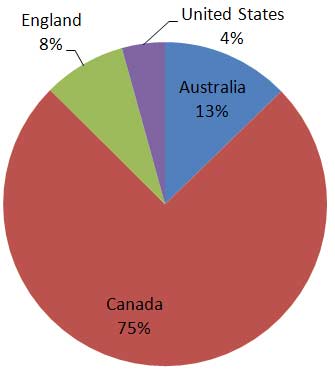
A pie chart should be used to show components that add up to a whole:

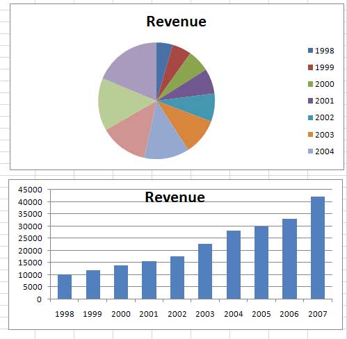
Never use a pie to show a time series. Instead, use a column or line chart:

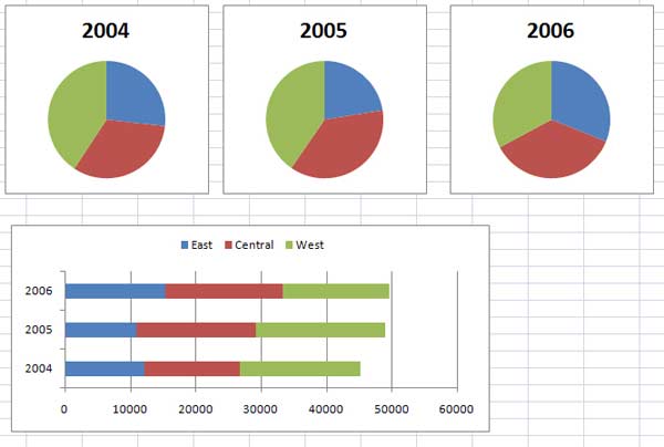
What if you need to show changing pies over time? Switch to a stacked bar chart:

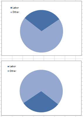
Avoid 3-D Pie charts. Which ever slice is in the front appears much larger. Here, both pies in this image have 30% for Labor, but the lower pie has 107% more dark blue pixels.

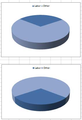
Instead, use a 2-D pie, where 30% looks like 30% whether it is at the top or the bottom:

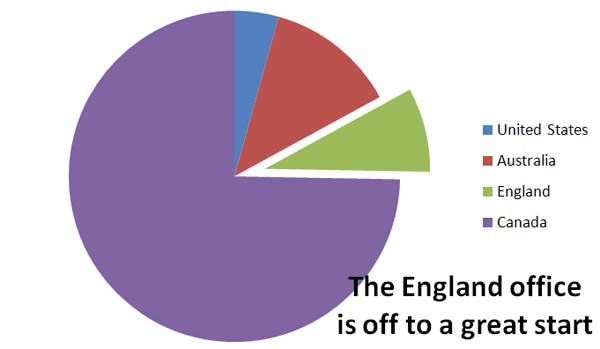
Rather than exploding the entire pie, it is more interesting to explode one slice of the pie. To do this, follow these steps:

• Create a regular (unexploded) pie chart.
• Click once on the pie. All wedges are selected.
• Click again on the desired wedge. Now, only that one data point is selected.
• Drag that wedge away from the center of the pie.

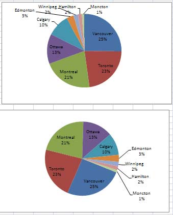
If you have many tiny slices, the labels tend to overwrite each other. Rotate the pie so that the small slices are in the lower right. There is more room for labels there. To rotate a pie chart:

• Right-click on the pie and choose Format Series
• In Excel 2007, the Angle of First Slice slider is first in the Series Options pane. In Excel 2003, click on the Options tab and change the Angle of First Slice.

In the top image, the labels are crowded at the top. In the bottom image, there are more room for the small slice labels:

If you have too many small slices, switch the chart type to a Bar of Pie type chart. Small slices are moved to a secondary chart:

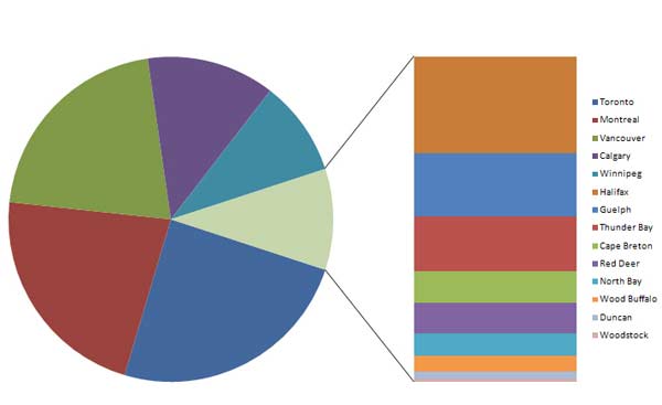
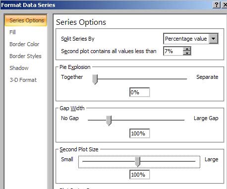
You can control which slices end up in the secondary pie. Right-click the pie and choose Format Data Series. The top options shown here allow you to specify that the secondary pie should be split by percentage, value, or number of items.