Summarize Excel Data

November 12, 2002 - by Bill Jelen

Bill asked this week's question about redundant Excel data.

I build a monthly transaction list in Excel. At the end of the month, I need to eliminate the redundant data and come up with a total by account code. Each account code can occur multiple times. Bill then described his current Excel methodology which is similar to method 1 below in order to come up with a unique list of account codes, with plans to use a matrix of CSE formulas to get the totals. He asks, is there an easier way to arrive at a unique list of account codes with totals for each account?

This is a perfect holiday question. Being a Lotus user for 15 years, I recognize Bill's method as the classic method for "quick-and-dirty" data manipulation from the good old days of Lotus release 2.1. This is a season to count our blessings. When you think about this question, you realize that the folks at Microsoft have really bestowed on us a number of tools over the years. If you are using Excel 97, there are at least five methods to do this task, all of which are far easier than the classic method described by Bill. I will offer a tutorial on the five methods this week.

My simplified data set has account numbers in column A and amounts in column B. The data runs from A2:B100. It is not sorted at the beginning.

Method 1

Use creative If statements in conjunction with Paste Special Values to find the answer.

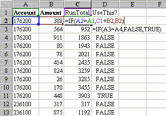
Given the newer tools offered by Excel, I no longer recommend this method. I used to use this a lot before better things came along and there are still situations where it comes in useful. My alternate name for this is "The-Lotus-123-When-You-Were-Not-In-The-Mood-To-Use-@DSUM" method. Here are the steps.

• Sort the data by column A.
• Invent a formula in column C which will keep a running total by account. Cell C2 is =IF(A2=A1,C1+B2,B2).
• Invent a formula in D which will identify the last entry for a particular account. Cell D2 is =IF(A2=A3,FALSE,TRUE).
• Copy C2:D2 down to all of your rows.
• Copy C2:D100. Do an Edit - PasteSpecial - Values back onto C2:D100 to change the formulae to values.
• Sort by column D descending.
• For the rows which have a TRUE in column D, you have a unique list of account numbers in A, and the final running total in C.

Pros: It is quick. All you need is a keen sense of writing IF statements.

Cons: There are better ways.

Method 2

Use Data Filter - Advanced Filter to get the list of unique accounts.

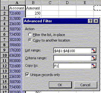
Bill's question was really how to get a unique list of account numbers so that he could use CSE Formulas to get the totals. This is a method for getting a list of the unique account numbers.

• Highlight A1:A100
• From the Menu, pick Data, Filter, Advanced Filter
• Click the radio button for "Copy to another location".
• Click the check box for "Unique Records Only".
• Pick a blank section of the worksheet where you want the unique list to appear. Enter this in the "Copy to:" field. (Note this field is greyed out until you pick "Copy to another location".
• Click OK. The unique account numbers will appear in F1.
• Enter any downline manipulations, array formulas, etc. to get your results.

Pros: Quicker than Method 1. No sorting required.

Cons: The CSE formulas required after this will make your head spin.

Method 3

Use Data Consolidate.

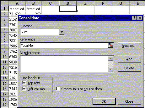
My quality of life improved when Excel offered Data Consolidate. This was BIG! It takes 30 seconds to set it up, but it spelled death for DSUMs and other methods.Your account number has to be to the left of the numeric fields you want to total. You have to have headings above each column. You need to assign a range name to the rectangular block of cells that include the account numbers along the left column and the headings along the top. In this case, that range is A1:B100.

• Highlight A1:B100
• Assign a range name to this area by clicking in the name box (to the left of the formula bar) and typing a name such as "TotalMe". (Alternately, use Insert - Name).
• Put the cell pointer in a blank section of the worksheet.
• Pick Data - Consolidate
• In the reference field, type the range name (TotalMe).
• In the Use Labels In section, check both Top Row and Left Column.
• Click OK

Pros: This is my favorite method. No sorting required. Shortcut is alt-D N (rangename) alt-T alt-L enter. It is easily scalable. If your range includes 12 monthly columns, the answer will have totals for each month.

Cons: If you do another Data Consolidate on the same sheet, you need to clear the old range name out of the All References field using the Delete button. The account number has to be to the left of your numeric data. It is slightly slower than pivot tables which becomes noticeable for datasets with 10,000+ records.

Method 4

Use Data Subtotals.

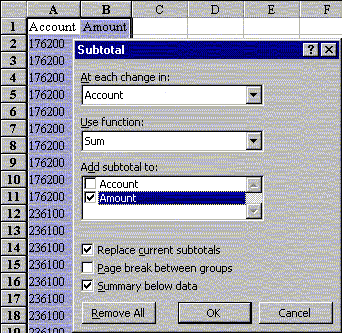
This is a cool feature. Because the resulting data is strange to work with, I use it less often than Data Consolidate.

• Sort by column A ascending.
• Select any cell in the data range.
• Choose Data - Subtotals from the menu.
• By default, Excel offers to subtotal the last column of your data. This works in this example, but you often have to scroll through the "Add Subtotal To:" list to pick the correct fields.
• Click OK. Excel will insert a new row at each change of account number with a total.

After you have the subtotals in, you will see a small 123 appear below the name box. Click on 2 to see just one line per account with the totals. Read Copy Excel Subtotals for an explanation of the special steps needed to copy these to a new location. Click on 3 to see all lines. Pros: Cool Feature. Great for printing reports with totals and pagebreaks after each section.

Cons: The data must be sorted first. Slow for lots of data. You have to use Goto-Special-VisbileCellsOnly to get the totals elsewhere. You have to use Data-Subtotals-RemoveAll to get back to your original data.

Method 5

Use a Pivot Table.

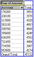
Pivot tables are the most versatile of all. Your data does not have to be sorted. The numeric columns can be to the left or right of the account number. You can easily have the account numbers go down or across the page.

• Select any cell in the data range.
• Choose Data - PivotTable from the menu.
• Accept the defaults in Step 1
• Make sure that the data range in step 2 is correct (it usually is)
• If you are using Excel 2000, click the Layout button on step 3. Excel 95 & 97 users automatically go to layout as step 3.
• In the layout dialog, drag the Account button from the right side of the dialog and drop it in the Row area.
• Drag the Amount button from the right side of the dialog and drop it in the Data area.
• Excel 2000 users click OK, Excel 95/97 users click Next.
• Specify if you want the results in a new sheet or in a specific section of an existing sheet. Read more about pivot tables in Excel Pivot Table Advanced Tricks.
• Pivot tables offer incredible functionality and make this task a snap. To copy the pivot table results, you need to do an Edit-PasteSpecial-Values, otherwise Excel will not let you insert rows, etc.

Pros: Quick, Flexible, Powerful. Fast, even for lots of data.

Cons: Somewhat intimidating.